1 · Working with behavioral data
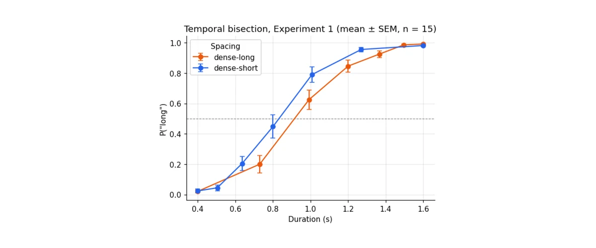
Load a temporal-bisection experiment, reshape it into tidy trials, aggregate it the right way, and draw the first psychometric curves.
15 October 2026
This series starts with phenomena that can be experienced and measured: biases in perceived time, limits of attention and memory, learning from prediction errors, and the representation of a stimulus in neural activity. Behavioral experiments turn those questions into data. Mathematical models make their assumptions explicit, and neural models ask how the same computation might be implemented.
Wherever possible, the examples use real timing and visual-search experiments from MSense Lab rather than generic benchmark tables. Learning rules are first written by hand in NumPy before a library implementation is introduced, so that the code does not conceal the mechanism.
The notebooks live in the
notebooks/foundations
folder of this site’s repository. Each page below is generated from the executed notebook, so the
figures are the notebook’s real output.
The explanations, derivations, code, simulations, and figures are developed specifically for this tutorial collection. Each topic follows the same scientific path:
You do not need advanced mathematics to begin, but four ideas recur throughout the series.
A trial is a vector when it contains one measurement per time point, and a matrix when it contains several variables or channels. I write a behavioral design matrix as \(X\in\mathbb{R}^{N\times P}\): \(N\) observations in rows and \(P\) predictors in columns. An EEG trial is usually \(X\in\mathbb{R}^{C\times T}\): \(C\) electrodes by \(T\) samples. Writing the shape beside every intermediate result is one of the simplest ways to prevent a correct formula from becoming incorrect code.
For a random variable \(Y\), \(\mathbb{E}[Y]\) is its long-run mean and \(\mathrm{Var}(Y)=\mathbb{E}[(Y-\mathbb{E}[Y])^2]\) measures dispersion. A probability model \(p(y\mid\theta)\) says how plausible an observation is under parameters \(\theta\). Statistical inference asks which parameter values are compatible with the observations and how uncertain those values remain.
For independent observations, the likelihood is
$$ L(\theta)=\prod_{i=1}^{N}p(y_i\mid\theta). $$Products are numerically awkward, so code normally minimizes the negative log-likelihood \(-\sum_i\log p(y_i\mid\theta)\). Squared error, binary cross-entropy, and multiclass cross-entropy are not unrelated recipes: each is a negative log-likelihood under a different observation model.
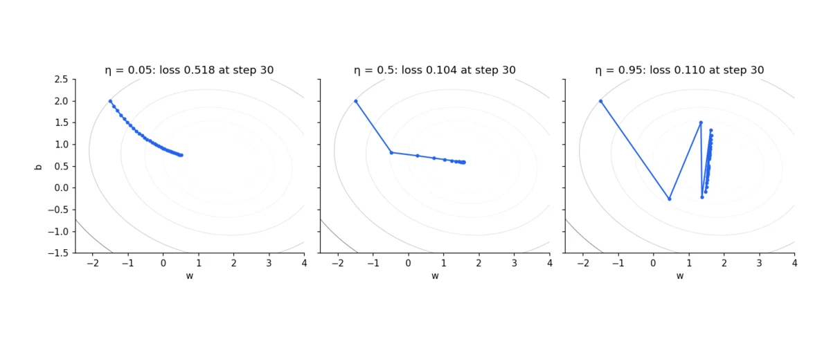
A derivative describes local sensitivity. The gradient \(\nabla_\theta\mathcal{L}\) collects the derivative of a loss with respect to every parameter. Gradient descent applies
$$ \theta_{k+1}=\theta_k-\eta\nabla_\theta\mathcal{L}(\theta_k), $$where \(\eta\) is the learning rate. Backpropagation is an efficient application of the chain rule for computing this gradient through a sequence of operations; it is not a separate learning principle.
Each notebook begins with a question, develops the minimum mathematics needed to answer it, implements the method, and ends by interpreting a result rather than treating code output as a conclusion.
Load a temporal-bisection experiment, reshape it into tidy trials, aggregate it the right way, and draw the first psychometric curves.
15 October 2026
Clean reaction times with a robust outlier rule, then build t-tests, permutation tests, and repeated-measures ANOVA from a visual-search experiment, checking each formula against a simulation.
15 October 2026
Derive least squares from a matrix equation, use it to measure the central-tendency effect in duration reproduction, and see why a mixed model is needed once trials are nested in participants.
15 October 2026
Fit psychometric functions by maximum likelihood written out by hand, add lapse rates, recover the bisection point and Weber fraction, and see that the same sigmoid is a single artificial neuron.
15 October 2026
McCulloch-Pitts threshold units, the perceptron learning rule and its XOR limit, Hebbian linear associators, and a Hopfield network that completes corrupted memories, all in a few lines of NumPy.
15 October 2026
Gradient descent on a loss surface, the delta rule, backpropagation derived and coded by hand and checked against PyTorch autograd, then overfitting, cross-validation, and an unsupervised competitive-learning contrast.
15 October 2026
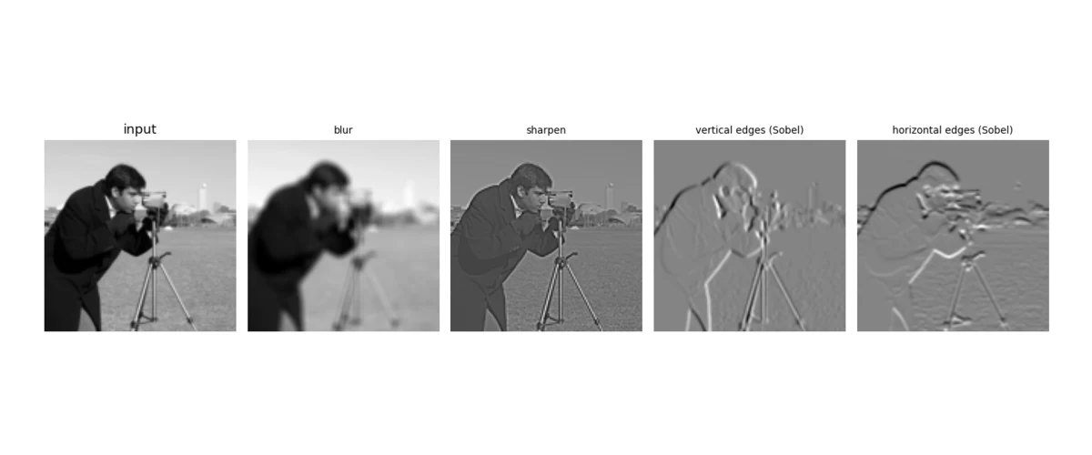
Convolution written by hand, Gabor filters as V1 receptive fields, an MLP versus a CNN on Fashion-MNIST, why weight sharing buys robustness to shifts, and transfer learning from twenty labeled examples per class.
15 October 2026
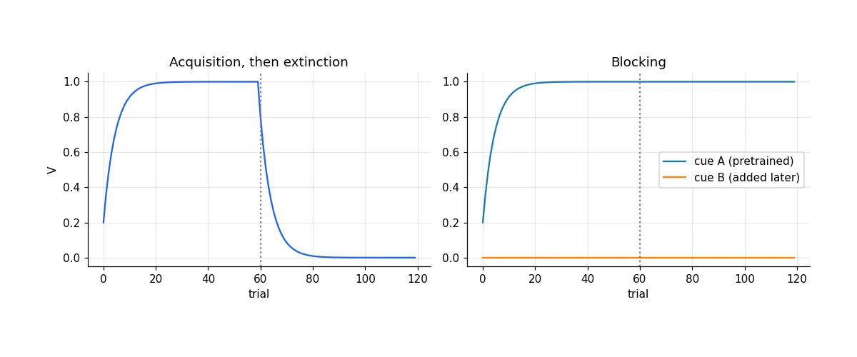
Rescorla-Wagner learning and blocking, temporal-difference errors that migrate from reward to cue like dopamine responses, value learning in a small maze, and an actor-critic agent that learns where to turn.
15 October 2026
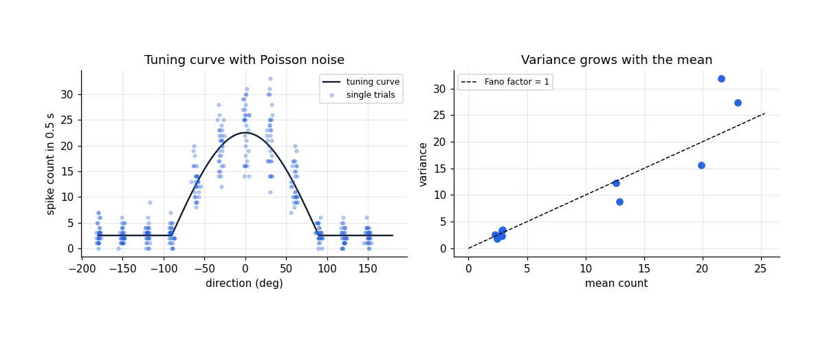
Poisson spiking and tuning curves, a linear-nonlinear neuron recovered by spike-triggered averaging, population-vector, maximum-likelihood, and Bayesian decoding, and how log-spaced duration tuning yields Weber's law.
15 October 2026
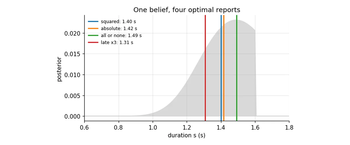
Probability on a grid, expected utility, and why the loss function decides which point of a belief gets reported. Then a timing case: reproduction with asymmetric feedback, where decision theory predicts a shift with no free parameters, and where mean and median observers turn out to be nearly impossible to tell apart.
16 October 2026
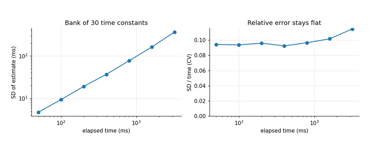
The leaky integrate-and-fire neuron from its equation: Euler steps, the f-I curve, the neuron as a linear filter, spike reliability, Poisson statistics, and integration versus coincidence detection. Then a timing case on two scales: one neuron can compare arrival times to microseconds, but cannot hold elapsed time for long. A bank of different time constants can, and it predicts Weber's law.
16 October 2026
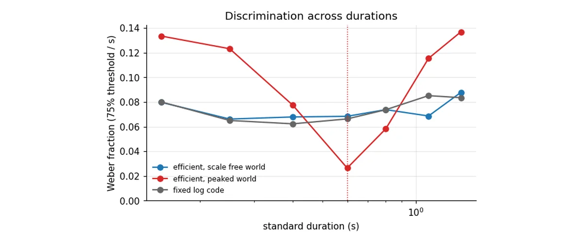
Entropy, mutual information, histogram equalization, Fisher information, and sparse coding, each computed and checked. Then a timing case: if neurons are allocated to durations by how often they occur, Weber's law follows from a scale-free world, and a peaked world should sharpen discrimination where durations are common. A local learning rule can build that code.
16 October 2026
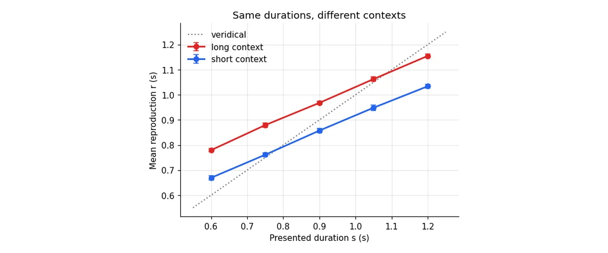
Bayes in log odds, conservatism, products of Gaussians, Weber's law from Fisher information, and neurons that add log likelihoods. Then the case: a duration feels longer among short ones. A reproduction experiment, a Bayesian observer and what the design can identify, a spiking implementation calibrated to behavior, a rival that fits equally well, and real data that break the constant noise assumption.
16 October 2026