Model Emergence

2 · Hypothesis testing by simulation and by formula

Clean reaction times with a robust outlier rule, then build t-tests, permutation tests, and repeated-measures ANOVA from a visual-search experiment, checking each formula against a simulation.

Open the notebook on GitHub →

A statistical test asks one question: if nothing interesting were going on, how surprising would data like mine be? Textbook formulas answer it analytically; a computer can answer it by brute force. This notebook does both for every test it introduces, so the formula never becomes a black box.

The experiment. Participants searched for a target among 8, 12, or 16 items and reported whether it was present. In the static condition the display stayed put; in the dynamic condition the items were relocated every 110 ms, so participants could not remember where they had already looked. The data are openly available at msenselab/dynamic_search.

import numpy as np
import pandas as pd
import matplotlib.pyplot as plt
from scipy import stats
import pingouin as pg

plt.rcParams.update({
    "figure.dpi": 110, "axes.spines.top": False, "axes.spines.right": False,
    "axes.grid": True, "grid.alpha": 0.3, "font.size": 10,
})
rng = np.random.default_rng(1)

raw = pd.read_csv("https://raw.githubusercontent.com/msenselab/dynamic_search/master/data/exp1.csv")
print(raw.head())
print(raw.groupby("sub").size().describe()[["count", "min", "max"]])

    target  setsize     dyn  resp        rt  sub  exp  correct
0   Absent       12  Static     2  2.583007    1    1        1
1   Absent        8  Static     2  0.935967    1    1        1
2  Present       16  Static     1  0.794771    1    1        1
3  Present        8  Static     1  1.241838    1    1        1
4   Absent       12  Static     2  1.759485    1    1        1
count     11.0
min      420.0
max      420.0
dtype: float64

Choosing a test

Which test fits depends on what kind of variable the outcome is and how the observations are grouped. The tests used in this series:

outcome	design	parametric	non-parametric / resampling
continuous	one group vs a value, or two paired conditions	one-sample / paired t-test	sign-flip permutation, Wilcoxon signed-rank
continuous	two independent groups	Welch t-test	label permutation, Mann-Whitney
continuous	several within-participant factors	repeated-measures ANOVA	permutation ANOVA, mixed models (notebook 3)
binary	any	logistic regression (notebook 4)
two continuous variables	association	Pearson r	Spearman ρ, permutation

Here every participant did every condition, so the comparisons are within-participant.

Cleaning reaction times

Reaction times are right-skewed and contain occasional lapses: anticipations, distraction, a finger resting on a key. A cut-off based on the mean and SD is itself distorted by the outliers it should detect. The median absolute deviation (MAD) is robust:

$$\mathrm{MAD} = 1.4826 \cdot \operatorname{median}\left(|x_i - \operatorname{median}(x)|\right)$$

The constant makes MAD equal the SD for normally distributed data. A common rule removes trials more than 3 MADs from the median, computed per participant and condition so that slow conditions are not penalised. We first drop timeouts (resp == -1) and errors.

def mad_outlier(x, k=3):
    med = np.median(x)
    mad = 1.4826 * np.median(np.abs(x - med))
    return np.abs(x - med) > k * mad

df = raw.query("resp != -1 and correct == 1").copy()
df["outlier"] = (df.groupby(["sub", "dyn", "target", "setsize"])["rt"]
                   .transform(lambda x: mad_outlier(x.to_numpy())))
print(f"timeouts and errors removed: {1 - len(df) / len(raw):.1%}; "
      f"MAD outliers among correct trials: {df['outlier'].mean():.1%}")

fig, axes = plt.subplots(1, 2, figsize=(9, 3.2), sharey=True)
for ax, (dyn, g) in zip(axes, df.groupby("dyn")):
    bins = np.linspace(0, 8, 60)
    ax.hist(g.loc[~g.outlier, "rt"], bins=bins, color="#2563eb", alpha=0.8, label="kept")
    ax.hist(g.loc[g.outlier, "rt"], bins=bins, color="#dc2626", label="MAD outlier")
    ax.set(title=f"{dyn} search", xlabel="RT (s)")
axes[0].set_ylabel("Trials")
axes[0].legend()
plt.tight_layout()
plt.show()

df = df.query("not outlier")

timeouts and errors removed: 6.6%; MAD outliers among correct trials: 2.9%

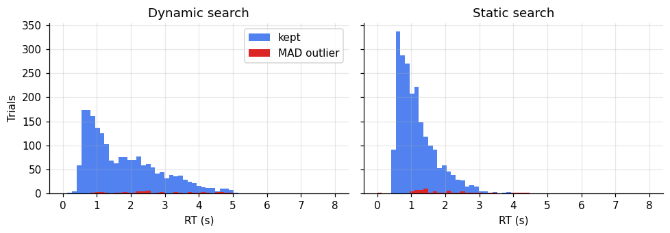
The distributions are clearly skewed, and dynamic search is both slower and more variable.

Paired t-test, by formula

Start with the simplest question: is target-present search slower in the dynamic condition? We aggregate to one mean RT per participant and condition, then take the difference $d_i$ for each participant. Under the null hypothesis the differences have mean zero, and

$$t = \frac{\bar d}{s_d / \sqrt{n}}$$

follows a t-distribution with $n-1$ degrees of freedom.

present = (df.query("target == 'Present'")
             .groupby(["sub", "dyn"])["rt"].mean().unstack())
d = present["Dynamic"] - present["Static"]
n = len(d)
t = d.mean() / (d.std(ddof=1) / np.sqrt(n))
p = 2 * stats.t.sf(abs(t), df=n - 1)
print(f"by hand: mean difference = {d.mean():.3f} s, t({n - 1}) = {t:.2f}, p = {p:.2g}")
print(stats.ttest_rel(present["Dynamic"], present["Static"]))

by hand: mean difference = 0.400 s, t(10) = 3.63, p = 0.0046
TtestResult(statistic=np.float64(3.628607313954578), pvalue=np.float64(0.0046232268929345755), df=np.int64(10))

The same test by simulation

Where does the t-distribution come from? Simulate it: draw $n$ differences from a population whose true mean is zero, compute $t$, repeat many times. The histogram of simulated $t$ values matches the analytic density, which is all the formula promises.

sims = rng.normal(0, 1, size=(20_000, n))
t_null = sims.mean(1) / (sims.std(1, ddof=1) / np.sqrt(n))

xs = np.linspace(-5, 5, 400)
fig, ax = plt.subplots(figsize=(6, 3.2))
ax.hist(t_null, bins=80, density=True, color="#94a3b8", label="simulated t under H0")
ax.plot(xs, stats.t.pdf(xs, n - 1), color="#2563eb", lw=2, label=f"t-distribution, df = {n - 1}")
ax.plot(xs, stats.norm.pdf(xs), color="#ea580c", ls="--", label="standard normal")
ax.set(xlabel="t", ylabel="density", title=f"Null distribution of t with n = {n}")
ax.legend(fontsize=8)
plt.show()
print(f"simulated P(|t| > 2.228) = {(np.abs(t_null) > 2.228).mean():.3f}  (analytic: 0.050)")

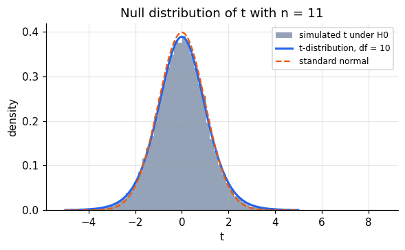
simulated P(|t| > 2.228) = 0.048  (analytic: 0.050)

The t-distribution has heavier tails than the normal because $s_d$ is itself estimated from only $n$ = 11 participants. Using a z-test here would make results look more significant than they are.

Permutation test: no distributional assumption

The t-test assumes the differences are roughly normal. A permutation test assumes only that, under the null, the condition labels are exchangeable within a participant. Swapping a participant’s two labels flips the sign of their difference, so the null distribution is obtained by randomly flipping signs.

def sign_flip_test(d, n_perm=20_000, rng=rng):
    d = np.asarray(d)
    flips = rng.choice([-1, 1], size=(n_perm, len(d)))
    null = (flips * d).mean(1)
    p = (np.sum(np.abs(null) >= abs(d.mean())) + 1) / (n_perm + 1)
    return p, null

p_perm, null = sign_flip_test(d)
fig, ax = plt.subplots(figsize=(6, 3))
ax.hist(null, bins=60, color="#94a3b8")
ax.axvline(d.mean(), color="#dc2626", lw=2, label=f"observed = {d.mean():.3f} s")
ax.set(xlabel="mean difference under sign flips (s)", ylabel="count",
       title=f"Sign-flip permutation test, p = {p_perm:.2g}")
ax.legend()
plt.show()
print(f"sign-flip p = {p_perm:.4f}; paired t-test p = {p:.4f}")

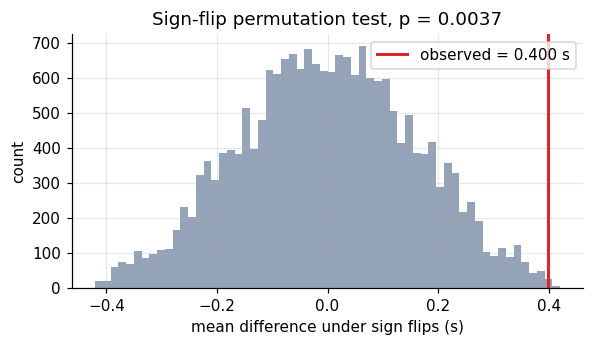
sign-flip p = 0.0037; paired t-test p = 0.0046

With 11 participants there are only $2^{11} = 2048$ distinct sign patterns, so the smallest attainable two-sided p-value is about 0.001. Ten of the eleven participants are slower in dynamic search, and the permutation p-value agrees closely with the t-test.

Effect size

A p-value says whether an effect is distinguishable from zero, not how large it is. For paired data a common standardised effect size is $d_z = \bar d / s_d$. The raw difference in seconds is often more informative still.

print(f"d_z = {d.mean() / d.std(ddof=1):.2f}")
print(pg.ttest(present["Dynamic"], present["Static"], paired=True)[["T", "dof", "p-val", "cohen-d", "BF10"]])

d_z = 1.09
               T  dof     p-val   cohen-d    BF10
T-test  3.628607   10  0.004623  1.301432  11.341

Note that pingouin’s cohen-d for paired data uses the pooled SD of the two conditions, not $s_d$, so it differs from $d_z$. Always say which one you report.

Repeated-measures ANOVA

The full design crosses dynamics (2) × set size (3) for target-present trials. The key quantity in visual search is the search slope: how much RT increases per additional item. A repeated-measures ANOVA tests the main effects and their interaction while partitioning out stable differences between participants.

cell = (df.query("target == 'Present'")
          .groupby(["sub", "dyn", "setsize"], as_index=False)["rt"].mean())

summary = cell.groupby(["dyn", "setsize"])["rt"].agg(["mean", "sem"]).reset_index()
fig, ax = plt.subplots(figsize=(5, 3.5))
for dyn, g in summary.groupby("dyn"):
    ax.errorbar(g["setsize"], g["mean"], yerr=g["sem"], marker="o", capsize=3, label=dyn)
ax.set(xlabel="Set size", ylabel="Mean RT (s)", xticks=[8, 12, 16],
       title="Target-present search (mean ± SEM)")
ax.legend()
plt.show()

aov = pg.rm_anova(data=cell, dv="rt", within=["dyn", "setsize"], subject="sub", detailed=True)
print(aov[["Source", "F", "ddof1", "ddof2", "p-unc", "ng2"]].round(4))

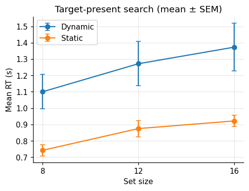
          Source        F  ddof1  ddof2   p-unc     ng2
0            dyn  13.1124      1     10  0.0047  0.3032
1        setsize  24.4292      2     20  0.0000  0.0870
2  dyn * setsize   1.4967      2     20  0.2479  0.0039

Both main effects are reliable: dynamic search is slower, and RT grows with set size. The interaction, which asks whether set size costs more in dynamic search, is not significant.

An interaction in an ANOVA is a difference of differences, and it is often clearer to compute the quantity it stands for directly. Here that is the per-participant search slope, from a straight line fitted to each participant’s three means, which turns the interaction into a paired test.

def slope(g):
    return np.polyfit(g["setsize"], g["rt"], 1)[0] * 1000  # ms per item

slopes = (cell.groupby(["sub", "dyn"]).apply(slope, include_groups=False)
              .unstack())
print(slopes.agg(["mean", "sem"]).round(1))
print(pg.ttest(slopes["Dynamic"], slopes["Static"], paired=True)[["T", "dof", "p-val"]])

dyn   Dynamic  Static
mean     34.1    22.4
sem       8.1     2.9
              T  dof     p-val
T-test  1.57614   10  0.146072

Dynamic slopes are larger on average (about 34 vs 22 ms per item), but they vary much more across participants, so with 11 people the difference is not reliable. This is the same conclusion as the interaction term, now in units one can interpret. Whether search “has memory” for visited locations would need more participants, or a model of the search process, to settle.

Correlation

Do participants who search slowly in static displays also search slowly in dynamic ones? A Pearson correlation across participants answers that, and again a permutation test, shuffling one variable relative to the other, shows what the p-value means.

x, y = present["Static"].to_numpy(), present["Dynamic"].to_numpy()
r = np.corrcoef(x, y)[0, 1]
null_r = np.array([np.corrcoef(x, rng.permutation(y))[0, 1] for _ in range(10_000)])
print(f"r = {r:.2f}, permutation p = {(np.abs(null_r) >= abs(r)).mean():.3f}, "
      f"scipy p = {stats.pearsonr(x, y).pvalue:.3f}")

fig, ax = plt.subplots(figsize=(4, 4))
ax.scatter(x, y, color="#2563eb")
ax.set(xlabel="Static RT (s)", ylabel="Dynamic RT (s)", title=f"r = {r:.2f}, n = {n}")
plt.show()

r = 0.53, permutation p = 0.095, scipy p = 0.090

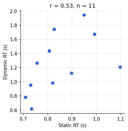
With 11 participants, a correlation needs to exceed about 0.6 to reach p < .05, so a correlation of 0.53 is suggestive at best, and its confidence interval is wide. Between-participant correlations need far more participants than within-participant effects.

Summary

Remove outliers with a robust rule (median ± 3 MAD) within participant and condition.
Aggregate to one value per participant and condition before testing within-participant effects.
A paired t-test is a one-sample test on differences; its null distribution can be simulated.
A sign-flip permutation test gives the same answer without assuming normality.
Report effect sizes, and say which effect size you report.
An ANOVA interaction is a difference of differences; computing the quantity it stands for, such as a search slope, makes it interpretable.

← Back to Model Emergence