Model Emergence

6 · How networks learn: gradients, backprop, and generalisation

Gradient descent on a loss surface, the delta rule, backpropagation derived and coded by hand and checked against PyTorch autograd, then overfitting, cross-validation, and an unsupervised competitive-learning contrast.

Open the notebook on GitHub →

Notebook 5 ended with a problem: a hidden layer can solve XOR, but the perceptron rule cannot find the hidden weights. This notebook solves it with gradient descent and backpropagation, the algorithm behind practically every trained neural network. Then it asks the question that matters more than training accuracy: does the network generalise to data it has not seen?

The three families of learning:

type	signal	example rule	notebook
supervised	a teacher gives the correct output	delta rule, backpropagation	here
unsupervised	input statistics only	Hebbian, competitive learning	5, here
reinforcement	delayed, scalar reward	temporal-difference learning	8

import numpy as np
import matplotlib.pyplot as plt
import torch
from sklearn.datasets import make_moons
from sklearn.model_selection import KFold

plt.rcParams.update({
    "figure.dpi": 110, "axes.spines.top": False, "axes.spines.right": False,
    "axes.grid": True, "grid.alpha": 0.3, "font.size": 10,
})
rng = np.random.default_rng(0)
_ = torch.manual_seed(0)

Gradient descent on a loss surface

Learning means choosing parameters that make a loss small. For a linear unit $\hat y = w x + b$ and mean squared error

$$L(w, b) = \frac1n \sum_i (\hat y_i - y_i)^2,$$

the gradient points uphill, so we step the other way: $\theta \leftarrow \theta - \eta\,\nabla_\theta L$. The learning rate $\eta$ controls the step size.

x = rng.uniform(-1, 1, 40)
y = 1.5 * x + 0.5 + rng.normal(0, 0.3, 40)

def loss(w, b):
    return np.mean((w * x + b - y) ** 2)

def grad(w, b):
    e = w * x + b - y
    return 2 * np.mean(e * x), 2 * np.mean(e)

def descend(eta, steps=30, start=(-1.5, 2.0)):
    w, b = start
    path = [(w, b)]
    for _ in range(steps):
        gw, gb = grad(w, b)
        w, b = w - eta * gw, b - eta * gb
        path.append((w, b))
    return np.array(path)

W, B = np.meshgrid(np.linspace(-2.5, 4, 200), np.linspace(-1.5, 2.5, 200))
Lgrid = np.mean((W[..., None] * x + B[..., None] - y) ** 2, axis=-1)

fig, axes = plt.subplots(1, 3, figsize=(12, 3.6), sharey=True)
for ax, eta in zip(axes, [0.05, 0.5, 0.95]):
    path = descend(eta)
    ax.contour(W, B, Lgrid, levels=Lgrid.min() + np.geomspace(0.01, 15, 14), cmap="Greys", linewidths=0.7)
    ax.plot(path[:, 0], path[:, 1], "o-", ms=3, color="#2563eb")
    ax.set(title=f"η = {eta}: loss {loss(*path[-1]):.3f} at step 30",
           xlabel="w", xlim=(-2.5, 4), ylim=(-1.5, 2.5))
    ax.grid(False)
axes[0].set_ylabel("b")
plt.tight_layout()
plt.show()

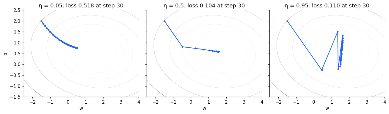
Too small a step crawls; a good step converges in a few iterations; too large a step overshoots and zig-zags across the valley. Here any $\eta$ above 1 makes the zig-zag grow instead of shrink, and the loss diverges. The limit is set by the curvature of the steepest direction. The surface here is a bowl because the model is linear; for neural networks it is not, but the update is the same.

The delta rule

Applying the update after every single example, rather than to the average loss, gives the delta rule (Widrow-Hoff, or least mean squares):

$$\Delta w_j = \eta\,(t - \hat y)\,x_j .$$

It looks like the perceptron rule but uses the continuous error $t - \hat y$. It is also the Rescorla-Wagner model of classical conditioning, where $t - \hat y$ is the prediction error that drives learning. Notebook 8 extends that error to predictions about the future.

Backpropagation

Take a network with one hidden layer of sigmoid units and a sigmoid output, trained with binary cross-entropy (notebook 4):

$$\mathbf h = \sigma(W_1\mathbf x + \mathbf b_1), \qquad \hat y = \sigma(\mathbf w_2^\top \mathbf h + b_2).$$

The chain rule gives every gradient by passing an error signal backwards. For sigmoid output with cross-entropy, the output error is simply $\delta_2 = \hat y - t$. Each hidden unit then receives its share of that error, weighted by its outgoing weight and scaled by its own slope:

$$\delta_1 = (\mathbf w_2\,\delta_2) \odot \mathbf h \odot (1 - \mathbf h).$$

The weight gradients are outer products of each layer’s error with its input, exactly as in the delta rule: $\nabla W_1 = \delta_1 \mathbf x^\top$ and $\nabla \mathbf w_2 = \delta_2\,\mathbf h$.

def sigmoid(z):
    return 1 / (1 + np.exp(-z))

class MLP:
    def __init__(self, n_in, n_hidden, rng=rng):
        self.W1 = rng.normal(0, 1, (n_hidden, n_in))
        self.b1 = np.zeros(n_hidden)
        self.w2 = rng.normal(0, 1, n_hidden)
        self.b2 = 0.0

    def forward(self, X):
        self.X = X
        self.H = sigmoid(X @ self.W1.T + self.b1)
        self.yhat = sigmoid(self.H @ self.w2 + self.b2)
        return self.yhat

    def loss(self, t):
        p = np.clip(self.yhat, 1e-9, 1 - 1e-9)
        return -np.mean(t * np.log(p) + (1 - t) * np.log(1 - p))

    def backward(self, t):
        n = len(t)
        d2 = (self.yhat - t) / n                          # output error
        d1 = np.outer(d2, self.w2) * self.H * (1 - self.H)  # hidden errors
        return {"w2": self.H.T @ d2, "b2": d2.sum(),
                "W1": d1.T @ self.X, "b1": d1.sum(0)}

    def step(self, grads, eta):
        for k, g in grads.items():
            setattr(self, k, getattr(self, k) - eta * g)

Xx = np.array([[0, 0], [0, 1], [1, 0], [1, 1]], float)
tx = np.array([0, 1, 1, 0], float)
net = MLP(2, 3)
losses = []
for epoch in range(5000):
    net.forward(Xx)
    losses.append(net.loss(tx))
    net.step(net.backward(tx), eta=1.0)
print("XOR outputs after training:", net.forward(Xx).round(3))

XOR outputs after training: [0.002 0.998 0.998 0.002]

The network has learned XOR, including hidden weights that the perceptron rule could not find.

Checking the gradients

A hand-derived gradient is easy to get subtly wrong. Two checks are standard: compare with a finite-difference estimate, and compare with automatic differentiation. PyTorch’s autograd records the forward computation and applies the chain rule for us.

net = MLP(2, 3)
net.forward(Xx)
analytic = net.backward(tx)

eps = 1e-6
numeric = np.zeros_like(net.W1)
for idx in np.ndindex(net.W1.shape):
    old = net.W1[idx]
    net.W1[idx] = old + eps; net.forward(Xx); lp = net.loss(tx)
    net.W1[idx] = old - eps; net.forward(Xx); lm = net.loss(tx)
    net.W1[idx] = old
    numeric[idx] = (lp - lm) / (2 * eps)

W1 = torch.tensor(net.W1, requires_grad=True)
b1 = torch.tensor(net.b1, requires_grad=True)
w2 = torch.tensor(net.w2, requires_grad=True)
b2 = torch.tensor(net.b2, requires_grad=True)
H = torch.sigmoid(torch.tensor(Xx) @ W1.T + b1)
yhat = torch.sigmoid(H @ w2 + b2)
torch.nn.functional.binary_cross_entropy(yhat, torch.tensor(tx)).backward()

print("max |analytic − finite difference|:", np.abs(analytic["W1"] - numeric).max())
print("max |analytic − autograd|:         ", np.abs(analytic["W1"] - W1.grad.numpy()).max())

max |analytic − finite difference|: 4.306338792503528e-11
max |analytic − autograd|:          1.0408340855860843e-17

All three agree to numerical precision. From here on we let autograd compute gradients.

Overfitting

A network with enough hidden units can fit almost any training set, including its noise. The real test is held-out data. The two moons dataset is a simple nonlinear problem; we give the network only 60 noisy training points.

Xm, tm = make_moons(n_samples=1060, noise=0.3, random_state=1)
X_train, t_train, X_test, t_test = Xm[:60], tm[:60], Xm[60:], tm[60:]

def make_net(hidden):
    return torch.nn.Sequential(torch.nn.Linear(2, hidden), torch.nn.Tanh(),
                               torch.nn.Linear(hidden, hidden), torch.nn.Tanh(),
                               torch.nn.Linear(hidden, 1))

def train(model, X, t, epochs=3000, lr=0.01, weight_decay=0.0, X_val=None, t_val=None):
    X, t = torch.tensor(X, dtype=torch.float32), torch.tensor(t, dtype=torch.float32)
    opt = torch.optim.Adam(model.parameters(), lr=lr, weight_decay=weight_decay)
    history = []
    for epoch in range(epochs):
        opt.zero_grad()
        loss = torch.nn.functional.binary_cross_entropy_with_logits(model(X).squeeze(1), t)
        loss.backward()
        opt.step()
        if X_val is not None and epoch % 25 == 0:
            history.append((loss.item(), evaluate(model, X_val, t_val)[0]))
    return history

@torch.no_grad()
def evaluate(model, X, t):
    X, t = torch.tensor(X, dtype=torch.float32), torch.tensor(t, dtype=torch.float32)
    logits = model(X).squeeze(1)
    loss = torch.nn.functional.binary_cross_entropy_with_logits(logits, t).item()
    acc = ((logits > 0).float() == t).float().mean().item()
    return loss, acc

torch.manual_seed(0)
big = make_net(64)
hist = np.array(train(big, X_train, t_train, X_val=X_test, t_val=t_test))

fig, axes = plt.subplots(1, 2, figsize=(10, 3.8))
ep = np.arange(len(hist)) * 25
axes[0].plot(ep, hist[:, 0], label="training loss")
axes[0].plot(ep, hist[:, 1], label="held-out loss")
axes[0].set(xlabel="epoch", ylabel="cross-entropy", yscale="log",
            title="Training loss falls, held-out loss turns up")
axes[0].legend()

gx, gy = np.meshgrid(np.linspace(-2, 3, 200), np.linspace(-1.5, 2, 200))
with torch.no_grad():
    zz = big(torch.tensor(np.c_[gx.ravel(), gy.ravel()], dtype=torch.float32)).reshape(gx.shape)
axes[1].contourf(gx, gy, torch.sigmoid(zz).numpy(), levels=20, cmap="RdBu_r", alpha=0.5)
axes[1].scatter(*X_train.T, c=t_train, cmap="RdBu_r", edgecolor="k", s=30)
axes[1].set(title="64 hidden units, 60 training points")
axes[1].grid(False)
plt.tight_layout()
plt.show()
print(f"train acc = {evaluate(big, X_train, t_train)[1]:.2f}, "
      f"held-out acc = {evaluate(big, X_test, t_test)[1]:.2f}")

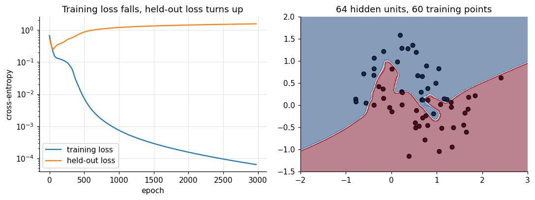
train acc = 1.00, held-out acc = 0.86

The boundary wraps around individual training points. Training loss keeps falling towards zero while held-out loss reaches a minimum and then rises: the network is memorising noise.

Three standard remedies are early stopping (halt near the held-out minimum), a smaller network, and weight decay, which adds $\lambda\lVert\mathbf w\rVert^2$ to the loss and so prefers smooth functions.

Choosing complexity by cross-validation

The held-out set must not be used to choose the model, or its error stops being an honest estimate. k-fold cross-validation chooses using the training data only: split it into $k$ folds, train on $k-1$, validate on the remaining one, rotate, and average.

def cv_loss(hidden, weight_decay, k=5, epochs=1500):
    losses = []
    for tr, va in KFold(k, shuffle=True, random_state=0).split(X_train):
        torch.manual_seed(0)
        m = make_net(hidden)
        train(m, X_train[tr], t_train[tr], epochs=epochs, weight_decay=weight_decay)
        losses.append(evaluate(m, X_train[va], t_train[va])[0])
    return np.mean(losses)

settings = [(h, wd) for h in (2, 8, 64) for wd in (0.0, 1e-2)]
scores = {s: cv_loss(*s) for s in settings}
for (h, wd), s in scores.items():
    print(f"hidden = {h:2d}, weight decay = {wd:<5}: CV loss = {s:.3f}")
best = min(scores, key=scores.get)
print("chosen:", best)

torch.manual_seed(0)
final = make_net(best[0])
train(final, X_train, t_train, epochs=1500, weight_decay=best[1])
print(f"held-out accuracy of chosen model: {evaluate(final, X_test, t_test)[1]:.2f} "
      f"(64 units, no decay, 3000 epochs: {evaluate(big, X_test, t_test)[1]:.2f})")

hidden =  2, weight decay = 0.0  : CV loss = 0.354
hidden =  2, weight decay = 0.01 : CV loss = 0.384
hidden =  8, weight decay = 0.0  : CV loss = 1.018
hidden =  8, weight decay = 0.01 : CV loss = 0.280
hidden = 64, weight decay = 0.0  : CV loss = 1.272
hidden = 64, weight decay = 0.01 : CV loss = 0.272
chosen: (64, 0.01)

held-out accuracy of chosen model: 0.91 (64 units, no decay, 3000 epochs: 0.86)

Cross-validation picks the setting from training data alone, and only then is the held-out set consulted, once. Notice what it chose: not the smallest network but the largest one with weight decay. Without decay, larger networks do worse; with it, extra capacity is harmless. How a network is constrained matters more than how big it is.

Unsupervised contrast: competitive learning

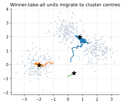
Without a teacher, a network can still discover structure. In competitive learning, output units compete for each input; only the winner, the unit whose weight vector is closest, moves its weights towards the input:

$$\mathbf w_{\text{win}} \leftarrow \mathbf w_{\text{win}} + \eta\,(\mathbf x - \mathbf w_{\text{win}}).$$

Each unit ends up at the centre of a cluster. This is online k-means, and a simple model of how feature detectors could self-organise.

centers = np.array([[-2, 0], [2, 1], [0, 2.5]])
Xu = np.vstack([rng.normal(c, 0.5, (150, 2)) for c in centers])
rng.shuffle(Xu)
Wc = rng.normal(0, 0.5, (3, 2))
trace = [Wc.copy()]
for x_ in Xu:
    win = np.argmin(((Wc - x_) ** 2).sum(1))
    Wc[win] += 0.05 * (x_ - Wc[win])
    trace.append(Wc.copy())
trace = np.array(trace)

fig, ax = plt.subplots(figsize=(5, 4))
ax.scatter(*Xu.T, s=6, color="#cbd5e1")
for j in range(3):
    ax.plot(trace[:, j, 0], trace[:, j, 1], lw=1.5)
    ax.plot(*trace[-1, j], "k*", ms=12)
ax.set(title="Winner-take-all units migrate to cluster centres")
plt.show()

Summary

Gradient descent steps against the gradient of a loss; the learning rate trades speed for stability.
The delta rule is gradient descent for a linear unit, and the Rescorla-Wagner rule in disguise.
Backpropagation passes errors backwards with the chain rule; check hand-written gradients against finite differences or autograd.
Training error says little about generalisation. Use held-out data, and choose complexity by cross-validation on the training set.
Competitive learning finds clusters without a teacher.

← Back to Model Emergence