Model Emergence

7 · Convolution, receptive fields, and transfer

Convolution written by hand, Gabor filters as V1 receptive fields, an MLP versus a CNN on Fashion-MNIST, why weight sharing buys robustness to shifts, and transfer learning from twenty labeled examples per class.

Open the notebook on GitHub →

A fully connected network treats an image as an unordered list of pixels. It does not know that neighbouring pixels belong together, or that a shoe is still a shoe when it moves three pixels to the left. Convolutional networks build both facts in, using the same two ideas the visual system uses: local receptive fields and the same detector repeated across space.

import numpy as np
import matplotlib.pyplot as plt
import torch
import torch.nn as nn
import torch.nn.functional as F
import torchvision
from scipy.signal import correlate2d
from skimage import data, transform

plt.rcParams.update({
    "figure.dpi": 110, "axes.spines.top": False, "axes.spines.right": False,
    "font.size": 10,
})
device = "cuda" if torch.cuda.is_available() else "cpu"
_ = torch.manual_seed(0)
print("device:", device)

device: cuda

Convolution by hand

A kernel is a small grid of weights. Slide it over the image; at each position, multiply the overlapping pixels by the weights and sum. Strictly this is cross-correlation (true convolution flips the kernel first), but deep learning libraries use the word convolution for it, and for learned kernels the distinction does not matter.

$$(I \star K)[i, j] = \sum_{u, v} I[i + u,\, j + v]\, K[u, v]$$

def conv2d(image, kernel):
    kh, kw = kernel.shape
    out = np.zeros((image.shape[0] - kh + 1, image.shape[1] - kw + 1))
    for i in range(out.shape[0]):
        for j in range(out.shape[1]):
            out[i, j] = np.sum(image[i:i + kh, j:j + kw] * kernel)
    return out

img = transform.resize(data.camera(), (128, 128), anti_aliasing=True)
kernels = {
    "blur": np.ones((5, 5)) / 25,
    "sharpen": np.array([[0, -1, 0], [-1, 5, -1], [0, -1, 0]]),
    "vertical edges (Sobel)": np.array([[-1, 0, 1], [-2, 0, 2], [-1, 0, 1]]),
    "horizontal edges (Sobel)": np.array([[-1, -2, -1], [0, 0, 0], [1, 2, 1]]),
}
print("matches scipy:", np.allclose(conv2d(img, kernels["sharpen"]),
                                    correlate2d(img, kernels["sharpen"], mode="valid")))

fig, axes = plt.subplots(1, 5, figsize=(13, 2.9))
axes[0].imshow(img, cmap="gray"); axes[0].set_title("input")
for ax, (name, k) in zip(axes[1:], kernels.items()):
    ax.imshow(conv2d(img, k), cmap="gray")
    ax.set_title(name, fontsize=9)
for ax in axes:
    ax.axis("off")
plt.tight_layout()
plt.show()

matches scipy: True

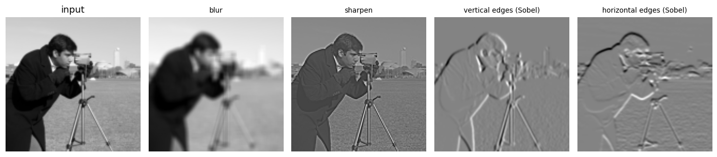
Each output pixel depends only on a small patch of the input, its receptive field, and the same kernel is applied everywhere. An edge detector that works in the top-left works in the bottom-right too.

Receptive fields in V1

Hubel and Wiesel found that simple cells in primary visual cortex respond to oriented edges and bars at a particular position. Their receptive fields are well described by Gabor functions: a sinusoidal grating under a Gaussian envelope. A bank of Gabor kernels at different orientations is a model of V1, and convolving with it gives an orientation-specific response map, one per orientation.

def gabor(theta, size=15, wavelength=6, sigma=3):
    r = np.arange(size) - size // 2
    x, y = np.meshgrid(r, r)
    xr = x * np.cos(theta) + y * np.sin(theta)
    g = np.exp(-(x ** 2 + y ** 2) / (2 * sigma ** 2)) * np.cos(2 * np.pi * xr / wavelength)
    return g - g.mean()

thetas = np.deg2rad([0, 45, 90, 135])
fig, axes = plt.subplots(2, 4, figsize=(10, 5))
for j, th in enumerate(thetas):
    k = gabor(th)
    axes[0, j].imshow(k, cmap="RdBu_r")
    axes[0, j].set_title(f"Gabor {np.rad2deg(th):.0f}°", fontsize=9)
    axes[1, j].imshow(np.abs(correlate2d(img, k, mode="valid")), cmap="magma")
for ax in axes.flat:
    ax.axis("off")
plt.tight_layout()
plt.show()

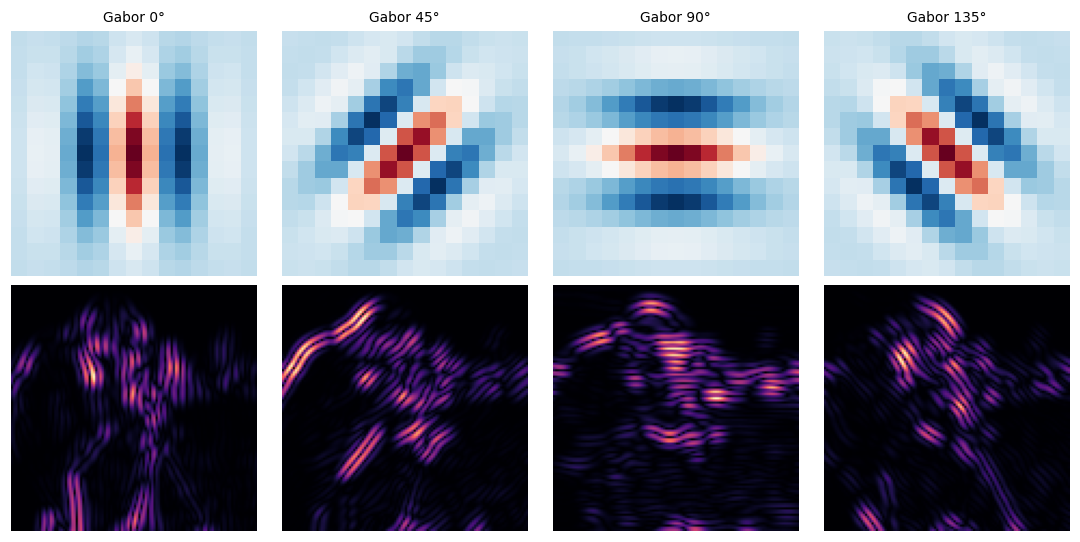
A CNN is not told to use Gabors. As we will see, it learns something similar from data.

Fashion-MNIST: MLP versus CNN

Fashion-MNIST has 70,000 grey-scale 28×28 images of clothing in 10 classes. It is a drop-in replacement for handwritten digits that is hard enough to separate good models from bad.

tf = torchvision.transforms.ToTensor()
train_set = torchvision.datasets.FashionMNIST("data", train=True, download=True, transform=tf)
test_set = torchvision.datasets.FashionMNIST("data", train=False, download=True, transform=tf)
classes = train_set.classes

X_train = train_set.data.float().div(255).unsqueeze(1)
y_train = train_set.targets
X_test = test_set.data.float().div(255).unsqueeze(1)
y_test = test_set.targets

fig, axes = plt.subplots(1, 10, figsize=(12, 1.6))
for c, ax in enumerate(axes):
    ax.imshow(X_train[y_train == c][0, 0], cmap="gray_r")
    ax.set_title(classes[c], fontsize=7)
    ax.axis("off")
plt.show()

Two models with a similar number of parameters. The MLP flattens the image; the CNN keeps it as a 2D grid and uses two convolution-pooling stages.

Conv2d(1, 16, 5) learns 16 kernels of size 5×5.
ReLU is the activation from notebook 4.
MaxPool2d(2) keeps the largest value in each 2×2 block, halving resolution and making the output tolerant to small shifts.
Finally a linear layer reads out the class.

mlp = nn.Sequential(nn.Flatten(), nn.Linear(784, 81), nn.ReLU(), nn.Linear(81, 10))

cnn = nn.Sequential(
    nn.Conv2d(1, 16, 5, padding=2), nn.ReLU(), nn.MaxPool2d(2),   # 16 × 14 × 14
    nn.Conv2d(16, 32, 5, padding=2), nn.ReLU(), nn.MaxPool2d(2),  # 32 × 7 × 7
    nn.Flatten(), nn.Linear(32 * 7 * 7, 32), nn.ReLU(), nn.Linear(32, 10))

def n_params(m):
    return sum(p.numel() for p in m.parameters())

print(f"MLP parameters: {n_params(mlp):,}")
print(f"CNN parameters: {n_params(cnn):,}")

MLP parameters: 64,405
CNN parameters: 63,786

def fit(model, X, y, epochs=5, lr=1e-3, batch=128, params=None):
    model.to(device)
    opt = torch.optim.Adam(params if params is not None else model.parameters(), lr=lr)
    n = len(X)
    for epoch in range(epochs):
        model.train()
        perm = torch.randperm(n)
        for i in range(0, n, batch):
            idx = perm[i:i + batch]
            xb, yb = X[idx].to(device), y[idx].to(device)
            opt.zero_grad()
            F.cross_entropy(model(xb), yb).backward()
            opt.step()
    return model

@torch.no_grad()
def accuracy(model, X, y):
    model.eval()
    preds = torch.cat([model(X[i:i + 2000].to(device)).argmax(1).cpu() for i in range(0, len(X), 2000)])
    return (preds == y).float().mean().item()

fit(mlp, X_train, y_train)
fit(cnn, X_train, y_train)
print(f"test accuracy  MLP: {accuracy(mlp, X_test, y_test):.3f}   CNN: {accuracy(cnn, X_test, y_test):.3f}")

test accuracy  MLP: 0.859   CNN: 0.886

With the same parameter budget, the CNN is clearly more accurate. Where the parameters go differs: the two convolutional layers together have only about 13,000 weights, because each kernel is shared across every position, and most of the CNN’s parameters sit in the readout.

What did it learn?

The first-layer kernels and the feature maps they produce for one image:

k1 = cnn[0].weight.detach().cpu()[:, 0]
x0 = X_test[:1].to(device)
with torch.no_grad():
    maps = cnn[1](cnn[0](x0))[0].cpu()

fig, axes = plt.subplots(2, 17, figsize=(13, 1.9))
axes[0, 0].imshow(X_test[0, 0], cmap="gray_r")
axes[0, 0].set_title("input", fontsize=8)
axes[1, 0].text(0.5, 0.5, "feature maps", ha="center", va="center", fontsize=8)
for j in range(16):
    lim = k1[j].abs().max()
    axes[0, j + 1].imshow(k1[j], cmap="RdBu_r", vmin=-lim, vmax=lim)
    axes[1, j + 1].imshow(maps[j], cmap="magma")
axes[0, 1].set_title("kernels →", fontsize=8, loc="left")
for ax in axes.flat:
    ax.axis("off")
plt.tight_layout()
plt.show()

At 5×5 pixels and after five epochs the kernels are rough, but several have an oriented light-dark structure, a coarse relative of the Gabors above, learned purely from the classification objective. The feature maps are easier to read: some respond to the outline of the boot, some to the sole, some to the filled interior.

Move every test image a few pixels sideways. The MLP has a separate weight for every pixel, so a shifted shoe activates entirely different weights. The CNN’s shared kernels respond to the feature wherever it is (equivariance), and pooling discards a little of the exact position.

shifts = [0, 1, 2, 3, 4]
acc_mlp = [accuracy(mlp, torch.roll(X_test, s, dims=3), y_test) for s in shifts]
acc_cnn = [accuracy(cnn, torch.roll(X_test, s, dims=3), y_test) for s in shifts]

fig, ax = plt.subplots(figsize=(5, 3.3))
ax.plot(shifts, acc_mlp, "o-", label="MLP")
ax.plot(shifts, acc_cnn, "o-", label="CNN")
ax.set(xlabel="horizontal shift (pixels)", ylabel="test accuracy",
       title="Robustness to translation", xticks=shifts)
ax.grid(alpha=0.3)
ax.legend()
plt.show()

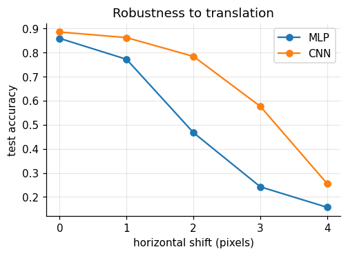
Both degrade, because Fashion-MNIST items are always centred during training, but the CNN degrades far more slowly. Training on randomly shifted, flipped, or rotated copies (data augmentation) closes much of the remaining gap by showing the network the variations it should ignore.

Transfer learning

Features learned for one task often help on another. Split the classes in two:

source task: T-shirt, trouser, pullover, dress, coat (all training images);
target task: sandal, shirt, sneaker, bag, ankle boot, with only 20 labelled images per class.

We compare four ways to learn the target task from those 100 images:

train a fresh CNN from scratch;
copy the source network, freeze the convolutional layers, and train the fully connected layers;
freeze everything except a new output layer (frozen up to the readout);
fine-tune all layers of the copied network with a small learning rate.

def make_cnn(n_out):
    return nn.Sequential(
        nn.Conv2d(1, 16, 5, padding=2), nn.ReLU(), nn.MaxPool2d(2),
        nn.Conv2d(16, 32, 5, padding=2), nn.ReLU(), nn.MaxPool2d(2),
        nn.Flatten(), nn.Linear(32 * 7 * 7, 32), nn.ReLU(), nn.Linear(32, n_out))

src_mask = y_train < 5
torch.manual_seed(0)
source = fit(make_cnn(5), X_train[src_mask], y_train[src_mask])

def target_split(n_per_class, seed):
    g = torch.Generator().manual_seed(seed)
    idx = torch.cat([torch.nonzero(y_train == c).squeeze(1)[torch.randperm(6000, generator=g)[:n_per_class]]
                     for c in range(5, 10)])
    return X_train[idx], y_train[idx] - 5

test_mask = y_test >= 5
Xt_test, yt_test = X_test[test_mask], y_test[test_mask] - 5

def from_source():
    m = make_cnn(5)
    m.load_state_dict(source.state_dict())
    m[-1] = nn.Linear(32, 5)          # new readout for the new classes
    return m

def frozen(up_to):
    m = from_source()
    for p in m[:up_to].parameters():
        p.requires_grad = False
    return m, [p for p in m.parameters() if p.requires_grad]

results = {"from scratch": [], "frozen conv": [], "frozen to readout": [], "fine-tuned": []}
for seed in range(5):
    Xs, ys = target_split(20, seed)
    torch.manual_seed(seed)
    results["from scratch"].append(accuracy(fit(make_cnn(5), Xs, ys, epochs=60, batch=32), Xt_test, yt_test))
    for name, up_to in [("frozen conv", 6), ("frozen to readout", 9)]:
        m, trainable = frozen(up_to)
        results[name].append(accuracy(fit(m, Xs, ys, epochs=60, batch=32, params=trainable), Xt_test, yt_test))
    results["fine-tuned"].append(accuracy(fit(from_source(), Xs, ys, epochs=60, batch=32, lr=3e-4),
                                          Xt_test, yt_test))

for k, v in results.items():
    print(f"{k:16s}: {np.mean(v):.3f} ± {np.std(v):.3f}  (5 random draws of 20 images per class)")

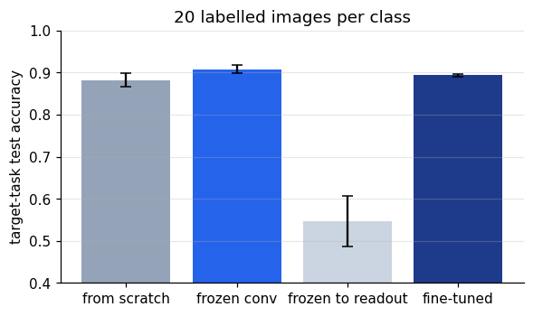
from scratch    : 0.882 ± 0.016  (5 random draws of 20 images per class)
frozen conv     : 0.908 ± 0.009  (5 random draws of 20 images per class)
frozen to readout: 0.547 ± 0.060  (5 random draws of 20 images per class)
fine-tuned      : 0.893 ± 0.003  (5 random draws of 20 images per class)

fig, ax = plt.subplots(figsize=(6, 3.3))
names = list(results)
ax.bar(names, [np.mean(results[k]) for k in names], yerr=[np.std(results[k]) for k in names],
       color=["#94a3b8", "#2563eb", "#cbd5e1", "#1e3a8a"], capsize=4)
ax.set(ylabel="target-task test accuracy", ylim=(0.4, 1), title="20 labelled images per class")
ax.grid(axis="y", alpha=0.3)
plt.show()

Two lessons, one small and one large.

The small one: reusing the frozen convolutional layers gives a modest but consistent gain over training from scratch, with less variability across draws of the 100 training images. The gain is small here because a tiny CNN already learns these 28×28 images well from 100 examples, and fine-tuning everything with a small learning rate lands in between.

The large one: freezing too much is a disaster. The fully connected hidden layer was tuned to separate T-shirts from pullovers, and its features do not separate sandals from sneakers. Early layers learn general features (edges, textures), later layers learn task-specific ones, so how much to transfer depends on how similar the tasks are. With natural images and networks pretrained on millions of photos, the general features are far richer and transfer is much more valuable, which is why ImageNet-pretrained networks are the usual starting point for small image datasets, and popular models of the ventral visual stream.

Summary

Convolution slides one small kernel over the whole image: local receptive fields and shared weights.
Gabor kernels model V1 simple cells; CNNs learn similar edge detectors on their own.
Shared weights make CNNs more accurate with fewer parameters and more robust to shifts.
Pooling and data augmentation add further tolerance to nuisance variation.
Transfer learning reuses features from a data-rich task to learn a data-poor one; early layers transfer, late layers often do not.

← Back to Model Emergence