Model Emergence
8 · Prediction errors: from conditioning to actor-critic
Rescorla-Wagner learning and blocking, temporal-difference errors that migrate from reward to cue like dopamine responses, value learning in a small maze, and an actor-critic agent that learns where to turn.
Supervised learning needs a teacher who knows the right answer. Animals rarely get one. They get rewards, often delayed, and must work out which of their earlier experiences and actions predicted them. Reinforcement learning formalises this, and its central quantity, the reward prediction error, turned out to be signalled by midbrain dopamine neurons.
The parts of an RL problem:
- a policy: which action to take in each state;
- a reward signal: what is good right now;
- a value function: how much reward to expect from a state onwards;
- optionally, a model of the environment for planning.
import numpy as np
import matplotlib.pyplot as plt

plt.rcParams.update({
    "figure.dpi": 110, "axes.spines.top": False, "axes.spines.right": False,
    "axes.grid": True, "grid.alpha": 0.3, "font.size": 10,
})
rng = np.random.default_rng(0)
Rescorla-Wagner: learning from surprise
In classical conditioning a cue (a bell) comes to predict an outcome (food). Rescorla and Wagner (1972) proposed that the associative strength \(V\) changes in proportion to the prediction error:
$$V \leftarrow V + \alpha\,(r - V).$$With several cues present, the prediction is the sum of their strengths, \(\hat r = \sum_j V_j\), and every present cue is updated by the same shared error. This is the delta rule from notebook 6 with cues as inputs.
def rescorla_wagner(cues, rewards, alpha=0.2):
    V = np.zeros(cues.shape[1])
    history = []
    for x, r in zip(cues, rewards):
        delta = r - x @ V
        V = V + alpha * delta * x
        history.append(V.copy())
    return np.array(history)

n = 60
# acquisition then extinction for a single cue
cues = np.ones((2 * n, 1))
rewards = np.r_[np.ones(n), np.zeros(n)]
h_single = rescorla_wagner(cues, rewards)

# blocking: A alone is rewarded, then A+B together
cues_block = np.r_[np.tile([1, 0], (n, 1)), np.tile([1, 1], (n, 1))]
h_block = rescorla_wagner(cues_block, np.ones(2 * n))

fig, axes = plt.subplots(1, 2, figsize=(10, 3.4))
axes[0].plot(h_single[:, 0], color="#2563eb")
axes[0].axvline(n, color="grey", ls=":")
axes[0].set(title="Acquisition, then extinction", xlabel="trial", ylabel="V")
axes[1].plot(h_block[:, 0], label="cue A (pretrained)")
axes[1].plot(h_block[:, 1], label="cue B (added later)")
axes[1].axvline(n, color="grey", ls=":")
axes[1].set(title="Blocking", xlabel="trial")
axes[1].legend()
plt.tight_layout()
plt.show()
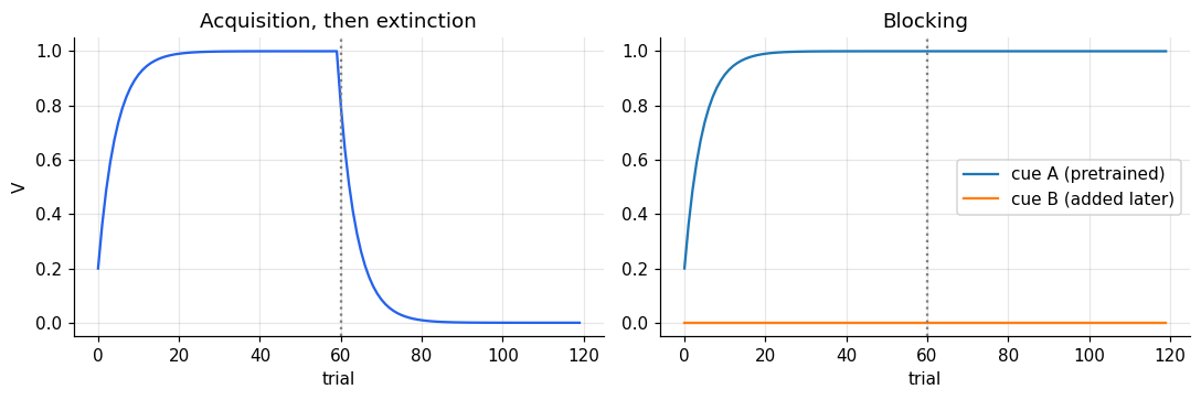
Blocking (Kamin, 1969) is the model’s signature prediction. Once cue A fully predicts the reward there is no error left, so cue B, though paired with reward on every trial, learns nothing. Learning is driven by surprise, not by co-occurrence, which is the key difference from Hebbian learning.
Predicting the future: temporal-difference learning
Rescorla-Wagner treats a trial as one moment. In reality a cue comes first and reward later, and the goal is to predict the total future reward from each moment,
$$V(t) = \mathbb E\Big[\sum_{\tau \ge 0} \gamma^\tau r(t + \tau)\Big].$$This obeys a recursion: \(V(t) = r(t) + \gamma V(t+1)\). Temporal-difference (TD) learning (Sutton, 1988) uses the mismatch in that recursion as its error,
$$\delta(t) = r(t) + \gamma V(t+1) - V(t),$$and updates the value of the current moment: \(V(t) \leftarrow V(t) + \alpha\,\delta(t)\). No need to wait for the future to arrive: each prediction is corrected by the next one.
To predict when reward arrives the model needs to know how much time has passed since the cue. The simplest assumption, the complete serial compound, gives each time step after the cue its own feature, like a tapped delay line.
T, cue_t, reward_t = 40, 10, 30
gamma, alpha, n_trials = 0.98, 0.3, 120

def run_td(n_trials, omit_on=()):
    # Feature k is active k steps after the cue; nothing is active before the cue, so the value
    # of pre-cue moments stays at zero and the cue itself is unpredicted.
    x = np.zeros((T, T))
    for t in range(cue_t, T):
        x[t, t - cue_t] = 1.0
    w = np.zeros(T)
    deltas = np.zeros((n_trials, T))
    for trial in range(n_trials):
        r = np.zeros(T)
        if trial not in omit_on:
            r[reward_t] = 1.0
        for t in range(T - 1):
            delta = r[t + 1] + gamma * (x[t + 1] @ w) - x[t] @ w
            deltas[trial, t + 1] = delta      # error on entering moment t + 1
            w += alpha * delta * x[t]
    return deltas

deltas = run_td(n_trials, omit_on={n_trials - 1})

fig, axes = plt.subplots(1, 2, figsize=(11, 3.6), gridspec_kw={"width_ratios": [1.3, 1]})
im = axes[0].imshow(deltas[:-1], aspect="auto", cmap="RdBu_r", vmin=-1, vmax=1,
                    extent=[0, T, n_trials - 1, 0])
axes[0].axvline(cue_t, color="k", lw=0.8)
axes[0].axvline(reward_t, color="k", lw=0.8, ls="--")
axes[0].set(xlabel="time step (cue at 10, reward at 30)", ylabel="trial",
            title="TD error across learning")
axes[0].grid(False)
fig.colorbar(im, ax=axes[0], label="δ")
for trial, lab, style in [(0, "trial 1", "-"), (n_trials - 1, "trained, reward omitted", "-"),
                          (n_trials - 2, "trained", "--")]:
    axes[1].plot(deltas[trial], ls=style, lw=2 if style == "--" else 1.5, label=lab)
axes[1].axvline(cue_t, color="grey", lw=0.8)
axes[1].axvline(reward_t, color="grey", lw=0.8, ls="--")
axes[1].set(xlabel="time step", ylabel="δ", title="Dopamine-like responses")
axes[1].legend(fontsize=8)
plt.tight_layout()
plt.show()
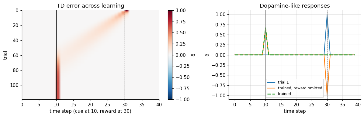
Early in learning, the error appears at the reward. As the value of the intervening moments is learned, the error moves back step by step until, after training, it appears at the cue, the first reliable predictor of reward, and has vanished at the reward itself. Omitting the reward on a trained trial gives a dip at exactly the time reward was due.
This is precisely what Schultz, Dayan and Montague (1997) found in dopamine neurons of the monkey ventral tegmental area. The dip on omission also shows that the system has learned when reward is due, not just whether. That depends on the time representation: with a tapped delay line timing is perfect, which real animals’ timing is not. Replacing it with representations that grow fuzzier with elapsed time (for example microstimuli, Ludvig, Sutton & Kehoe, 2008) connects TD learning to the scalar variability of interval timing.
Values of states: a rat in a barn
Now let the agent move. A rat starts at A and turns left or right, reaching B or C; there it turns again and receives a reward.
           A
         /   \
        B     C
       / \   / \
      0   5 2   0
Under a random policy (each turn left or right with probability 0.5) the true values are \(v(B) = 0.5\cdot0 + 0.5\cdot5 = 2.5\), \(v(C) = 0.5\cdot2 + 0.5\cdot0 = 1\), and \(v(A) = 0.5\,v(B) + 0.5\,v(C) = 1.75\). TD learning should find them from experience alone.
maze = {"A": {"L": ("B", 0.0), "R": ("C", 0.0)},
        "B": {"L": (None, 0.0), "R": (None, 5.0)},
        "C": {"L": (None, 2.0), "R": (None, 0.0)}}

def td_policy_evaluation(n_episodes=300, alpha=0.1):
    v = {"A": 0.0, "B": 0.0, "C": 0.0}
    trace = []
    for _ in range(n_episodes):
        s = "A"
        while s is not None:
            a = rng.choice(["L", "R"])
            s_next, r = maze[s][a]
            v_next = v[s_next] if s_next else 0.0
            v[s] += alpha * (r + v_next - v[s])
            s = s_next
        trace.append(dict(v))
    return trace

trace = td_policy_evaluation()
fig, ax = plt.subplots(figsize=(5.5, 3.4))
for s, true in [("A", 1.75), ("B", 2.5), ("C", 1.0)]:
    line, = ax.plot([t[s] for t in trace], label=f"v({s})")
    ax.axhline(true, color=line.get_color(), ls=":", lw=1)
ax.set(xlabel="episode", ylabel="value estimate", title="TD learning under a random policy")
ax.legend()
plt.show()
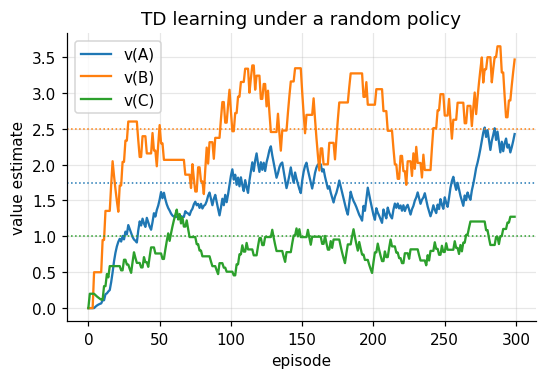
The estimates converge to the true values (dotted) and keep fluctuating around them, because with a constant learning rate every new random reward nudges them.
Learning to act: actor-critic
Knowing values is not the same as acting well. In an actor-critic architecture two systems share one error signal:
- the critic learns state values with TD, \(v(s) \leftarrow v(s) + \alpha_c\,\delta\);
- the actor keeps a preference \(m(s, a)\) for each action and chooses by softmax, \(P(a \mid s) = \dfrac{e^{\beta m(s,a)}}{\sum_b e^{\beta m(s,b)}}\), where the inverse temperature \(\beta\) trades exploitation against exploration;
- after each step, the action just taken is reinforced if the outcome was better than the critic expected: \(m(s, a) \leftarrow m(s, a) + \alpha_a\,\delta\).
The critic and actor are often mapped onto ventral and dorsal striatum, with dopamine broadcasting \(\delta\) to both.
def actor_critic(n_episodes=400, alpha_c=0.1, alpha_a=0.1, beta=1.0):
    v = {s: 0.0 for s in maze}
    m = {s: {"L": 0.0, "R": 0.0} for s in maze}
    p_trace = []
    for _ in range(n_episodes):
        s = "A"
        while s is not None:
            prefs = np.array([m[s]["L"], m[s]["R"]])
            p = np.exp(beta * prefs) / np.exp(beta * prefs).sum()
            a = "L" if rng.random() < p[0] else "R"
            s_next, r = maze[s][a]
            delta = r + (v[s_next] if s_next else 0.0) - v[s]
            v[s] += alpha_c * delta
            m[s][a] += alpha_a * delta
            s = s_next
        p_trace.append({s: 1 / (1 + np.exp(-beta * (m[s]["L"] - m[s]["R"]))) for s in maze})
    return p_trace, v

p_trace, v_final = actor_critic()
fig, ax = plt.subplots(figsize=(5.5, 3.4))
for s in maze:
    ax.plot([p[s] for p in p_trace], label=f"P(left | {s})")
ax.set(xlabel="episode", ylabel="probability", ylim=(-0.02, 1.02),
       title="Actor-critic learns where to turn")
ax.legend()
plt.show()
print("final critic values:", {s: round(x, 2) for s, x in v_final.items()})
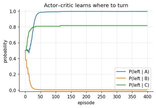
final critic values: {'A': 5.0, 'B': 5.0, 'C': 1.49}
The agent learns to turn left at A and right at B, the route to the large reward. As the policy improves, the critic’s values rise from the random-policy values towards those of the good policy (\(v(A)\) and \(v(B)\) approach 5). At C the agent should turn left, but because it rarely visits C once it prefers B, that preference is learned slowly: what an agent knows depends on where its own policy takes it.
Summary
- Rescorla-Wagner learning is driven by prediction error and explains blocking.
- TD learning predicts future reward and corrects each prediction with the next one.
- TD errors move from reward to the earliest predictive cue and dip on omission, like dopamine neurons; this requires a representation of elapsed time.
- TD learning estimates state values from experience; an actor-critic uses the same error to improve its policy.