Model Emergence
10 · What problem is the brain solving?
Probability on a grid, expected utility, and why the loss function decides which point of a belief gets reported. Then a timing case: reproduction with asymmetric feedback, where decision theory predicts a shift with no free parameters, and where mean and median observers turn out to be nearly impossible to tell apart.
A model of behavior has to say what the behavior is for. Before asking how neurons estimate a duration, we need to know what counts as a good estimate. Reporting the most likely value is one answer. Reporting the average is another. They are not the same, and the data can tell them apart only under some designs.
This unit has two parts.
Part I · Foundations builds the tools: probability on a grid, Bayes’ rule, expected utility, loss functions, the cost of exact inference, and resource limits. Every formula comes with its code line and the shape of the array it produces.
Part II · Case study uses those tools on one timing question, in six stages:
| stage | question |
|---|---|
| 1. Cognitive phenomenon | What needs explaining? |
| 2. Behavioral experiment | How do we make it measurable? |
| 3. Empirical signature | What pattern in the data is the phenomenon? |
| 4. Computational model | What computation produces it, and can we identify it? |
| 5. Neural implementation | Could neurons carry it out? |
| 6. Prediction and failure | Which result would prove the model wrong? |
All data here are simulated from models whose parameters we set. That way every analysis can be checked against the truth.
import numpy as np
import matplotlib.pyplot as plt
from scipy.ndimage import gaussian_filter1d
from scipy.optimize import minimize
from scipy.stats import norm

plt.rcParams.update({
    "figure.dpi": 110, "axes.spines.top": False, "axes.spines.right": False,
    "axes.grid": True, "grid.alpha": 0.3, "font.size": 10,
})
rng = np.random.default_rng(0)
1. Three questions about one behavior
Marr (1982) split the explanation of any information processing system into three questions. They are easiest to see on a concrete task. A participant sees a flash lasting \(s\) seconds and then holds a key for the same time.
| level | the question | for duration reproduction |
|---|---|---|
| computational | What is being computed, and why is it the right thing? | Choose a key press that keeps the expected error small, given what is known about \(s\). |
| algorithmic | Which representation and which steps? | Combine a noisy measurement with knowledge of the usual durations, then read out one number. |
| implementational | Which physical substrate? | Duration tuned neurons, an integrator, a motor command. |
The levels constrain each other but do not determine each other. Many algorithms solve one computational problem, and many circuits run one algorithm. This unit stays mostly at the first level. Its point is that the computational level is testable: different goals predict different behavior.
2. Probability on a grid
We represent every belief as a vector of probabilities over a grid of possible values. Integrals become sums, and every step is a line of NumPy.
The symbols, with what they mean in the task:
| symbol | meaning | array | shape |
|---|---|---|---|
| \(s\) | the true duration on a trial | s_grid | (K,) |
| \(m\) | the noisy internal measurement of that duration | m_grid | (M,) |
| \(p(s)\) | the prior: how often each duration occurs in the experiment | prior | (K,) |
| \(p(m \mid s)\) | the likelihood: how measurements scatter around a given duration | lik | (K, M) |
For timing, measurement noise grows with the duration (Gibbon, 1977). A convenient way to get that is Gaussian noise on a log scale:
$$\log m = \log s + \varepsilon, \qquad \varepsilon \sim \mathcal N(0, \sigma_w^2).$$Here \(\sigma_w\) is the Weber fraction: the size of the noise relative to the duration.
K, M = 241, 200
s_grid = np.linspace(0.2, 2.2, K)                       # (K,) candidate durations, s
m_grid = np.exp(np.linspace(np.log(0.15), np.log(3.5), M))  # (M,) possible measurements, m
sigma_w = 0.15                                          # Weber fraction

prior = ((s_grid >= 0.4) & (s_grid <= 1.6)).astype(float)
prior /= prior.sum()                                    # (K,) uniform on 0.4 to 1.6 s

# p(m | s): one row per duration, one column per measurement
lik = norm.pdf(np.log(m_grid)[None, :], np.log(s_grid)[:, None], sigma_w)
lik /= lik.sum(axis=1, keepdims=True)                   # (K, M), each row sums to 1

print("prior", prior.shape, " likelihood", lik.shape)
print("rows of p(m|s) sum to", lik.sum(axis=1)[:3].round(6))
prior (241,)  likelihood (241, 200)
rows of p(m|s) sum to [1. 1. 1.]
Three rules turn these pieces into a belief about \(s\) after seeing \(m\).
| rule | formula | code | shape |
|---|---|---|---|
| joint | \(p(s, m) = p(m \mid s)\,p(s)\) | joint = lik * prior[:, None] | (K, M) |
| marginal | \(p(m) = \sum_s p(s, m)\) | p_m = joint.sum(axis=0) | (M,) |
| posterior | \(p(s \mid m) = p(s, m) / p(m)\) | post = joint / p_m | (K, M) |
The last line is Bayes’ rule. Each column of post is the belief about the duration after one
particular measurement.
joint = lik * prior[:, None]          # (K, M)  p(s, m)
p_m = joint.sum(axis=0)               # (M,)    p(m), how often each measurement occurs
post = joint / p_m                    # (K, M)  p(s | m), one column per measurement

print("joint sums to", joint.sum().round(6))
print("posterior columns sum to", post.sum(axis=0)[[50, 100, 150]].round(6))

j = np.argmin(np.abs(m_grid - 1.5))
fig, axes = plt.subplots(1, 2, figsize=(9, 3.4))
axes[0].pcolormesh(m_grid, s_grid, joint, shading="auto", cmap="Greys")
axes[0].axvline(m_grid[j], color="C3", lw=1.5)
axes[0].set(xlabel="measurement m (s)", ylabel="duration s (s)", title="joint p(s, m)", xlim=(0.2, 2.5))
axes[1].plot(s_grid, post[:, j], color="C3")
axes[1].plot(s_grid, prior / prior.max() * post[:, j].max(), color="0.6", ls="--", label="prior (scaled)")
axes[1].set(xlabel="duration s (s)", ylabel="probability", title=f"posterior given m = {m_grid[j]:.2f} s")
axes[1].legend(frameon=False)
plt.tight_layout()
plt.show()
joint sums to 1.0
posterior columns sum to [1. 1. 1.]
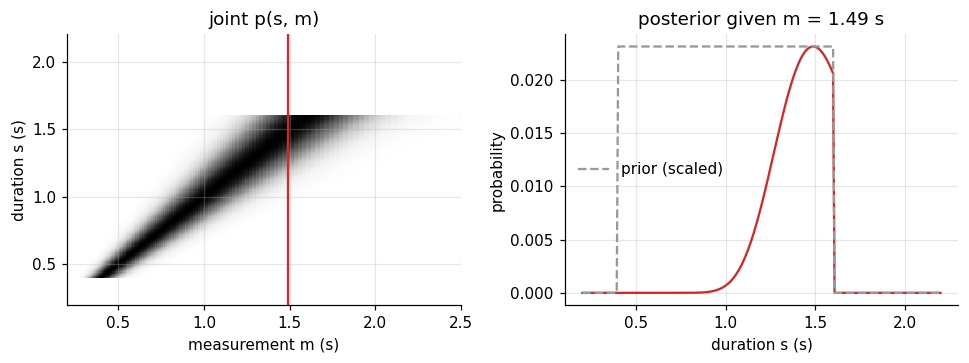
The red column in the joint distribution, renormalized, is the posterior on the right. Two things shape it. Log noise makes beliefs wider for longer durations. The prior ends at 1.6 s and cuts the belief off sharply on the right, so the belief is lopsided: a steep wall on one side, a slope on the other. Both features will matter.
3. Decisions: states, signals, actions, utility
A belief is not yet a behavior. Bayesian decision theory (Wald, 1950) adds three ingredients.
| symbol | meaning in the task | array | shape |
|---|---|---|---|
| \(a\) | the action: how long the key is held | a_grid | (A,) |
| \(\pi(a \mid m)\) | the policy: which action to take after measurement \(m\) | policy | (M, A) |
| \(u(s, a)\) | the utility: how good action \(a\) is when the duration was \(s\) | util | (K, A) |
The expected utility of an action, given a measurement, averages the utility over the posterior:
$$\bar u(a \mid m) = \sum_s p(s \mid m)\, u(s, a).$$In code this is one matrix product, EU = post.T @ util, with shape (M, A). The best policy picks,
for each measurement, the action with the largest expected utility.
We start with the utility most experiments imply when they give points for accuracy: minus the squared error, \(u(s, a) = -(a - s)^2\).
a_grid = s_grid.copy()                                  # (A,) possible key presses, A = K here
util = -(a_grid[None, :] - s_grid[:, None]) ** 2        # (K, A) utility u(s, a)

EU = post.T @ util                                      # (M, A) expected utility of each action
best_a = a_grid[EU.argmax(axis=1)]                      # (M,)   the optimal action per measurement
policy = np.zeros((M, K)); policy[np.arange(M), EU.argmax(axis=1)] = 1   # (M, A) deterministic policy

# Value of the whole policy: average over measurements, actions, and states
value = (p_m[:, None] * policy * EU).sum()
print(f"expected utility of the optimal policy: {value:.4f}  (mean squared error {-value:.4f} s^2)")

# Check by brute force: simulate trials and score them
n = 200_000
s_sim = rng.choice(s_grid, size=n, p=prior)
m_sim = s_sim * np.exp(rng.normal(0, sigma_w, n))
a_sim = np.interp(m_sim, m_grid, best_a)
print(f"simulated mean squared error:            {np.mean((a_sim - s_sim) ** 2):.4f} s^2")
expected utility of the optimal policy: -0.0169  (mean squared error 0.0169 s^2)
simulated mean squared error:            0.0169 s^2
The two numbers agree. The grid calculation and a simulation of 200,000 trials give the same answer, so the formula means what we said it means.
4. The loss decides which point of the belief you report
Utility is often written as a loss, \(L = -u\). A short calculation shows which action minimizes each common loss. Set the derivative of the expected loss to zero:
| loss \(L(a, s)\) | what it punishes | optimal action | code |
|---|---|---|---|
| \((a - s)^2\) | large errors much more than small ones | posterior mean | post_j @ s_grid |
| \(\lvert a - s \rvert\) | all errors in proportion | posterior median | first s where cdf >= 0.5 |
| \(\mathbb 1[a \neq s]\) | any error at all, equally | posterior mode | s_grid[post_j.argmax()] |
| \(c_\text{late}(a-s)\) if late, \(c_\text{early}(s-a)\) if early | late and early errors differently | posterior quantile \(q = \frac{c_\text{early}}{c_\text{early} + c_\text{late}}\) | first s where cdf >= q |
The last row needs one line of algebra. The expected loss is
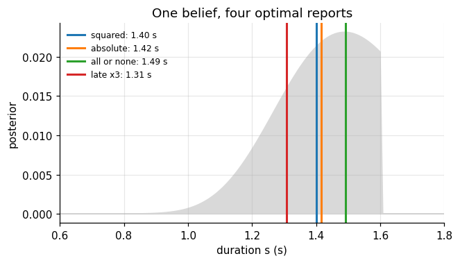
\(c_\text{late} \sum_{s Below we check each row numerically: brute force search over actions must land on the formula. One belief gives four different reports, spread over almost 0.2 s. The mode sits near the
measurement. The median and the mean are pulled away from the wall, and the quantile lies lower
still. Nothing about the perception changed. Only the goal changed. This is why a model of reproduction must state its
loss: a bias in the reports may come from the belief, from the loss, or from both. The grid above has \(K = 241\) values for one duration. Real inference problems involve many
variables at once. Suppose the brain wanted a joint belief about the durations of the last \(N\)
trials, which it would need if one trial’s estimate depends on the others. The joint grid has
\(K^N\) cells. Ten trials on a coarse grid already need more memory than exists. The difficulty is the
normalizer \(p(m) = \sum_s p(m \mid s)p(s)\): it sums over every combination. Brains, and our models
of them, must therefore approximate. Later units cover the two main families, sampling and
variational methods. The design principles are the same everywhere: break the problem into parts,
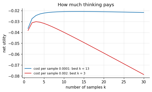
reuse computation, sample instead of enumerating, and follow gradients. Two classical results explain why decision theory leans on probability. Real agents also pay for computation. Resource rationality asks for the best policy among those
that respect a cost (Lieder & Griffiths, 2020): A clean example: instead of computing the posterior mean, draw \(k\) samples from the posterior and
average them. If the posterior variance is \(\sigma^2\), the estimate itself has variance \(\sigma^2/k\),
so the expected squared error is \(\sigma^2(1 + 1/k)\). With a cost \(c\) per sample, the net utility is When samples are expensive relative to the uncertainty, one sample is optimal (Vul et al., 2014). When people reproduce durations, their reports drift toward the middle of the range they have
been shown: short intervals come out too long, long ones too short (Hollingworth, 1910;
Jazayeri & Shadlen, 2010). Part I showed that a reported number is a belief plus a goal.
So the phenomenon has two possible sources, and we want to know how much each contributes. The question for this case: when people reproduce a duration, which summary of their belief do
they report, and do they change it when the payoffs change? In pointing tasks people adjust
their aim to asymmetric penalties close to optimally (Trommershäuser, Maloney & Landy, 2003), and
the shape of the loss they minimize can be measured (Körding & Wolpert, 2004). We ask the same of
timing. Each trial shows one of seven durations from 0.4 to 1.6 s, then the participant holds a key to
reproduce it. Two blocks differ only in the feedback: The design logic: the stimuli and the prior are identical, so any difference between blocks must
come from the loss. We simulate a participant who is exactly optimal: mean in the symmetric block, the 0.25 quantile in
the asymmetric block. The participant also has motor noise \(\sigma_\text{mot}\): the hand does not
release the key exactly when intended. An optimal agent should take that into account too. With
asymmetric costs, the quantile is taken of the belief convolved with its own motor noise. Before any model, describe the data. Two numbers per duration: the mean reproduction in each block,
and the difference between the blocks. Three facts describe the data: The third fact is the useful one. A participant who simply “presses a bit earlier” would produce a
flat line. Any model has to explain why longer durations move more. The model is Part I applied to the task. Three steps per trial, each with a free or fixed
quantity: The likelihood of one reproduction sums over the measurements the participant might have had: In code: The shift in Stage 3 now has an explanation. The quantile sits further below the mean when the
belief is wide, and log noise makes the belief wider for longer durations. The model also predicts
the fall at the top: near 1.6 s the prior edge cuts the belief off and narrows it, so the shift
should level off or drop there. The mean observer fits best and recovers both noise parameters. But look at the median observer:
its fit is close, and it pays for the wrong rule by moving its noise parameters. The mode observer
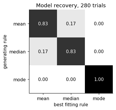
is clearly worse. One data set is not enough to trust this ranking, so we run the standard check. Model recovery. Simulate many data sets from each rule, fit all three rules to each, and count
how often the generating rule wins. The mode is identified every time. Mean and median are confused in one data set out of six, even
though the simulated participants differ in nothing but the rule. Their predictions differ only
where the belief is lopsided, and there by less than the trial to trial noise. This is the failure case of the symmetric block. It cannot reliably tell us whether the timer
minimizes squared or absolute error. Here the simulated participant is perfectly stationary and has
no lapses; real data would blur the small difference further. More trials of the same kind buy
little, because the two rules only disagree on the few trials where the belief hits the prior edge.
A better design makes the candidate losses disagree strongly. The asymmetric block does that for a
different question: not mean versus median, but whether a changed loss is used at all. Fit \(\sigma_w\) and \(\sigma_\text{mot}\) on the symmetric block only. Then decision theory fixes the
asymmetric block completely: the quantile is \(q = 1/(1+3) = 0.25\), taken of the belief convolved with
the fitted motor noise. Nothing is refitted. The predicted curve follows the data without having seen the asymmetric block. No point misses it
by more than about two standard errors; the largest miss is at 1.2 s. The curve also bends down at
the top, as Stage 4 said it would. Keep them apart. So far we have only the first. Can neurons compute a quantile? Reading out a mean needs a weighted sum. A quantile needs something
else: a running total of belief, compared with a threshold. Reproduction tasks offer a natural
circuit for that. With \(\theta = 0.5\) the circuit releases at the median; with \(\theta = 0.25\) at the 0.25 quantile.
Changing the payoff only needs to change one number, the threshold. The gain was chosen so that the population fires only a few spikes per trial, which makes the
decoded belief about as wide as the behavioral Weber fraction. With that one calibration the
circuit reproduces the ideal observer’s shift: growing with duration, bending down at the prior
edge. With more spikes the belief narrows and the shift shrinks. That is a second, independent
prediction: a participant whose timing is more precise should show a smaller payoff shift. This establishes only that the computation is implementable. Ramping activity that reaches a
threshold at the moment of a timed response is a well known pattern in timing tasks, but the
simulation does not show that any brain area does this. A causal claim would need an intervention:
for example, a manipulation that changes the threshold and moves reproductions by the amount the
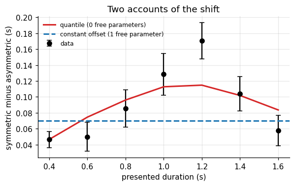
model predicts, without changing their variability. The model makes claims that could be false. Each one names the result that would reject it. Below we test the first row against its natural rival: a participant who has learned a constant
offset \(\delta\), \(a = \text{mean} - \delta\). The rival gets one free parameter, fitted on half of the
asymmetric trials. Both models are scored on the other half. Here the quantile model wins on held out trials, with one parameter fewer. That is the expected
outcome, because the data were generated by it. What makes the test worth running on real people
is that it can fail. Three ways it could:post_j = post[:, j] # (K,) one skewed posterior
cdf = post_j.cumsum() # (K,) P(s <= value)
losses = {
"squared": (a_grid[None, :] - s_grid[:, None]) ** 2,
"absolute": np.abs(a_grid[None, :] - s_grid[:, None]),
"all or none": (np.abs(a_grid[None, :] - s_grid[:, None]) > 0.005).astype(float),
"late x3": np.where(a_grid[None, :] > s_grid[:, None],
3 * (a_grid[None, :] - s_grid[:, None]),
1 * (s_grid[:, None] - a_grid[None, :])),
}
formula = {
"squared": post_j @ s_grid,
"absolute": s_grid[np.searchsorted(cdf, 0.5)],
"all or none": s_grid[post_j.argmax()],
"late x3": s_grid[np.searchsorted(cdf, 0.25)],
}
fig, ax = plt.subplots(figsize=(6.5, 3.4))
ax.fill_between(s_grid, post_j, color="0.85")
for (name, Lmat), col in zip(losses.items(), ["C0", "C1", "C2", "C3"]):
exp_loss = post_j @ Lmat # (A,) expected loss of each action
a_star = a_grid[exp_loss.argmin()]
print(f"{name:12s} brute force {a_star:.3f} s formula {formula[name]:.3f} s")
ax.axvline(a_star, color=col, lw=2, label=f"{name}: {a_star:.2f} s")
ax.set(xlabel="duration s (s)", ylabel="posterior", xlim=(0.6, 1.8), title="One belief, four optimal reports")
ax.legend(frameon=False, fontsize=8)
plt.show()
squared      brute force 1.400 s   formula 1.400 s
absolute     brute force 1.417 s   formula 1.417 s
all or none  brute force 1.492 s   formula 1.492 s
late x3      brute force 1.308 s   formula 1.308 s
5. Why exact inference gets expensive
K_small = 50                                            # a coarse grid: 50 levels per duration
for N in [1, 2, 3, 5, 10, 20]:
    cells = float(K_small) ** N
    gigabytes = cells * 8 / 1e9
    print(f"N = {N:2d} trials: {cells:.1e} cells, {gigabytes:.1e} GB as float64")
N =  1 trials: 5.0e+01 cells, 4.0e-07 GB as float64
N =  2 trials: 2.5e+03 cells, 2.0e-05 GB as float64
N =  3 trials: 1.2e+05 cells, 1.0e-03 GB as float64
N =  5 trials: 3.1e+08 cells, 2.5e+00 GB as float64
N = 10 trials: 9.8e+16 cells, 7.8e+08 GB as float64
N = 20 trials: 9.5e+33 cells, 7.6e+25 GB as float64
6. Why Bayes, and what limits it
var_post = post_j @ (s_grid - post_j @ s_grid) ** 2     # scalar posterior variance
ks = np.arange(1, 31)                                   # (k,) number of samples

# Check the error formula by simulation
k_test, reps = 4, 100_000
truth = rng.choice(s_grid, size=reps, p=post_j)         # (reps,) the duration, drawn from the belief
est = rng.choice(s_grid, size=(reps, k_test), p=post_j).mean(axis=1)   # (reps,) k-sample estimate
print(f"posterior variance {var_post:.4f}; error with k={k_test}: "
      f"formula {var_post * (1 + 1 / k_test):.4f}, simulation {np.mean((est - truth) ** 2):.4f}")

fig, ax = plt.subplots(figsize=(6, 3.3))
for c, col in [(1e-4, "C0"), (2e-3, "C3")]:
    U = -var_post * (1 + 1 / ks) - c * ks               # (k,) net utility
    ax.plot(ks, U, color=col, label=f"cost per sample {c:g}: best k = {ks[U.argmax()]}")
ax.set(xlabel="number of samples k", ylabel="net utility", title="How much thinking pays")
ax.legend(frameon=False, fontsize=8)
plt.show()
posterior variance 0.0181; error with k=4: formula 0.0226, simulation 0.0226
What Part I gives us
Part II · Case study: which loss does a timer minimize?
Stage 1 · Cognitive phenomenon
Stage 2 · Behavioral experiment
durs = np.round(np.linspace(0.4, 1.6, 7), 2)            # (D,) the presented durations
n_per = 60                                              # trials per duration per block
ds = s_grid[1] - s_grid[0]


def posterior(sw):
    # p(s | m) for every m on the grid, as rows: (M, K)
    L = norm.pdf(np.log(m_grid)[:, None], np.log(s_grid)[None, :], sw)
    P = L * prior[None, :]
    return P / P.sum(axis=1, keepdims=True)


def readout(P, rule, s_mot=0.0, q=0.25):
    # Map each measurement to an intended action: (M,)
    if rule == "mean":
        return P @ s_grid
    if rule == "mode":
        return s_grid[P.argmax(axis=1)]
    if s_mot > 0:                                       # belief about the outcome includes motor noise
        P = gaussian_filter1d(P, s_mot / ds, axis=1, mode="constant")
        P = P / P.sum(axis=1, keepdims=True)
    level = {"median": 0.5, "quantile": q}[rule]
    idx = (P.cumsum(axis=1) < level).sum(axis=1)
    return s_grid[np.minimum(idx, K - 1)]


def simulate(rule, sw, s_mot, q=0.25, n=n_per):
    a_of_m = readout(posterior(sw), rule, s_mot, q)    # (M,)
    s = np.repeat(durs, n)                              # (N,) true durations
    m = s * np.exp(rng.normal(0, sw, s.size))           # (N,) measurements
    r = np.interp(m, m_grid, a_of_m) + rng.normal(0, s_mot, s.size)   # (N,) key presses
    return s, r


true_sw, true_mot = 0.15, 0.05
s_sym, r_sym = simulate("mean", true_sw, true_mot)
s_asy, r_asy = simulate("quantile", true_sw, true_mot, q=0.25)
print("symmetric block:", s_sym.shape, " asymmetric block:", s_asy.shape)
symmetric block: (420,) asymmetric block: (420,)
Stage 3 · Empirical signature
mean_sym = np.array([r_sym[s_sym == d].mean() for d in durs])      # (D,)
mean_asy = np.array([r_asy[s_asy == d].mean() for d in durs])      # (D,)
shift = mean_sym - mean_asy                                         # (D,) how much earlier
se_shift = np.array([np.sqrt(r_sym[s_sym == d].var() / n_per + r_asy[s_asy == d].var() / n_per)
                     for d in durs])

fig, axes = plt.subplots(1, 2, figsize=(9.5, 3.5))
axes[0].plot(durs, durs, color="0.7", ls="--", label="veridical")
axes[0].plot(durs, mean_sym, "o-", color="C0", label="symmetric feedback")
axes[0].plot(durs, mean_asy, "o-", color="C3", label="late costs 3x")
axes[0].set(xlabel="presented duration (s)", ylabel="mean reproduction (s)", title="Reproductions")
axes[0].legend(frameon=False, fontsize=8)
axes[1].errorbar(durs, shift, yerr=se_shift, fmt="o-", color="k", capsize=3)
axes[1].axhline(0, color="0.7")
axes[1].set(xlabel="presented duration (s)", ylabel="symmetric minus asymmetric (s)",
            title="How much earlier with asymmetric costs")
plt.tight_layout()
plt.show()
slope_sym = np.polyfit(durs, mean_sym, 1)[0]
print(f"slope of reproduction on duration (symmetric): {slope_sym:.2f}")
(b, b0), cov = np.polyfit(durs, shift, 1, w=1 / se_shift, cov="unscaled")
print("shift per duration (s):", shift.round(3))
print(f"slope of shift on duration: {b:.3f} +/- {np.sqrt(cov[0, 0]):.3f} s per s")
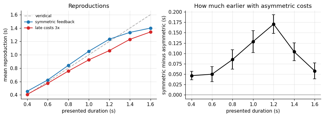
slope of reproduction on duration (symmetric): 0.83
shift per duration (s): [0.046 0.05  0.085 0.129 0.17  0.104 0.058]
slope of shift on duration: 0.048 +/- 0.015 s per s
Stage 4 · Computational model
step formula meaning parameter measure \(\log m = \log s + \varepsilon\) noisy sense of duration \(\sigma_w\), free infer \(p(s \mid m) \propto p(m \mid s)\,p(s)\) belief after one trial none: the prior is the experiment’s range act \(a = \) mean, median, mode, or quantile of the belief the loss being minimized the rule execute \(r = a + \eta,\; \eta \sim \mathcal N(0, \sigma_\text{mot}^2)\) imprecise release \(\sigma_\text{mot}\), free W has shape (N, M), the action table a_of_m has shape (M,), and the sum is a row sum.def neg_log_lik(theta, s, r, rule, q=0.25):
sw, s_mot = np.exp(theta) # fit on log scale to keep both positive
a_of_m = readout(posterior(sw), rule, s_mot if rule == "quantile" else 0.0, q) # (M,)
W = norm.pdf(np.log(m_grid)[None, :], np.log(s)[:, None], sw)
W /= W.sum(axis=1, keepdims=True) # (N, M) p(m | s) for each trial
like = (W * norm.pdf(r[:, None], a_of_m[None, :], s_mot)).sum(axis=1) # (N,)
return -np.log(like + 1e-300).sum()
def fit(s, r, rule, q=0.25):
res = minimize(neg_log_lik, np.log([0.1, 0.1]), args=(s, r, rule, q), method="Nelder-Mead",
options={"xatol": 1e-3, "fatol": 1e-3})
return np.exp(res.x), res.fun
for rule in ["mean", "median", "mode"]:
(sw_hat, mot_hat), nll = fit(s_sym, r_sym, rule)
print(f"{rule:6s} sigma_w = {sw_hat:.3f} sigma_mot = {mot_hat:.3f} -log L = {nll:7.1f}")
print(f"truth sigma_w = {true_sw:.3f} sigma_mot = {true_mot:.3f} (rule: mean)")
mean sigma_w = 0.154 sigma_mot = 0.043 -log L = -351.7
median sigma_w = 0.173 sigma_mot = 0.038 -log L = -344.5
mode    sigma_w = 0.125  sigma_mot = 0.070   -log L =  -265.3
truth   sigma_w = 0.150  sigma_mot = 0.050   (rule: mean)
rules = ["mean", "median", "mode"]
n_rep = 6
confusion = np.zeros((3, 3))                            # rows: generating rule, columns: winning rule
for g, gen in enumerate(rules):
    for _ in range(n_rep):
        s_g, r_g = simulate(gen, true_sw, true_mot)
        nlls = [fit(s_g, r_g, rule)[1] for rule in rules]
        confusion[g, int(np.argmin(nlls))] += 1
confusion /= n_rep
print(confusion.round(2))

fig, ax = plt.subplots(figsize=(4.2, 3.4))
im = ax.imshow(confusion, cmap="Greys", vmin=0, vmax=1)
for i in range(3):
    for k in range(3):
        ax.text(k, i, f"{confusion[i, k]:.2f}", ha="center", va="center",
                color="w" if confusion[i, k] > 0.5 else "k")
ax.set(xticks=range(3), xticklabels=rules, yticks=range(3), yticklabels=rules,
       xlabel="best fitting rule", ylabel="generating rule", title="Model recovery, 280 trials")
ax.grid(False)
plt.show()
[[0.83 0.17 0.  ]
 [0.17 0.83 0.  ]
 [0.   0.   1.  ]]
A prediction with no free parameters
(sw_hat, mot_hat), _ = fit(s_sym, r_sym, "mean")
a_mean = readout(posterior(sw_hat), "mean")             # (M,)
a_q = readout(posterior(sw_hat), "quantile", mot_hat, q=0.25)   # (M,)


def predicted_means(a_of_m, sw):
    W = norm.pdf(np.log(m_grid)[None, :], np.log(durs)[:, None], sw)
    W /= W.sum(axis=1, keepdims=True)                   # (D, M)
    return W @ a_of_m                                   # (D,) expected reproduction per duration


pred_shift = predicted_means(a_mean, sw_hat) - predicted_means(a_q, sw_hat)   # (D,)
fig, ax = plt.subplots(figsize=(6, 3.4))
ax.errorbar(durs, shift, yerr=se_shift, fmt="o", color="k", capsize=3, label="data")
ax.plot(durs, pred_shift, color="C3", lw=2, label="decision theory, zero free parameters")
ax.set(xlabel="presented duration (s)", ylabel="symmetric minus asymmetric (s)",
       title="The shift was predicted before it was fitted")
ax.legend(frameon=False, fontsize=8)
plt.show()
print("predicted shift:", pred_shift.round(3))
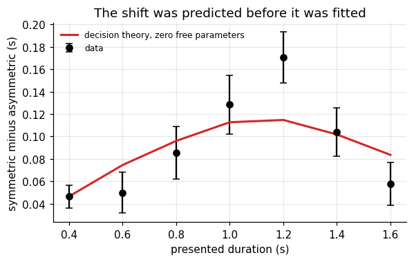
predicted shift: [0.047 0.075 0.096 0.113 0.115 0.102 0.084]
Three levels of claim
claim what supports it what we have here consistent with the model reproduces the data pattern yes, including a parameter free prediction implementable a plausible circuit can compute it Stage 5 causal changing the mechanism changes behavior as predicted not addressed by behavior alone Stage 5 · Neural implementation
n_neur = 40
pref = np.exp(np.linspace(np.log(0.25), np.log(2.5), n_neur))       # (I,) preferred durations
width, gain = 0.25, 0.3                                              # tuning width (log units), expected peak count

f = gain * np.exp(-0.5 * ((np.log(s_grid)[:, None] - np.log(pref)[None, :]) / width) ** 2)   # (K, I)
log_f = np.log(f + 1e-12)


def neural_release(s_true, theta, n_trials=400):
    counts = rng.poisson(gain * np.exp(-0.5 * ((np.log(s_true) - np.log(pref)) / width) ** 2),
                         size=(n_trials, n_neur))                    # (T, I) spike counts
    log_post = counts @ log_f.T - f.sum(axis=1) + np.log(prior + 1e-300)   # (T, K)
    p = np.exp(log_post - log_post.max(axis=1, keepdims=True))
    p /= p.sum(axis=1, keepdims=True)                                # (T, K) belief per trial
    C = p.cumsum(axis=1)                                             # (T, K) accumulated belief as t grows
    return s_grid[(C < theta).sum(axis=1)]                           # (T,) release times


# How wide is the decoded belief? Compare with the behavioral Weber fraction.
cnt = rng.poisson(gain * np.exp(-0.5 * ((np.log(1.0) - np.log(pref)) / width) ** 2), size=(2000, n_neur))
lp = cnt @ log_f.T - f.sum(axis=1)                                   # flat prior: width from the code alone
pp = np.exp(lp - lp.max(axis=1, keepdims=True)); pp /= pp.sum(axis=1, keepdims=True)
mu = pp @ np.log(s_grid)
sd_log = np.sqrt((pp * (np.log(s_grid)[None, :] - mu[:, None]) ** 2).sum(axis=1)).mean()
print(f"spikes per trial: {cnt.sum(axis=1).mean():.1f}; width of decoded belief: {sd_log:.3f} log units "
      f"(behavioral sigma_w {true_sw})")


fig, ax = plt.subplots(figsize=(6, 3.4))
ax.plot(durs, durs, color="0.7", ls="--")
rel = {}
for theta, col in [(0.5, "C0"), (0.25, "C3")]:
    rel[theta] = np.array([neural_release(d, theta).mean() for d in durs])
    ax.plot(durs, rel[theta], "o-", color=col, label=f"threshold {theta}")
ax.set(xlabel="presented duration (s)", ylabel="mean release time (s)",
       title="One circuit, two payoffs, one changed number")
ax.legend(frameon=False, fontsize=8)
plt.show()
print("neural shift (theta 0.5 minus 0.25):", (rel[0.5] - rel[0.25]).round(3))
spikes per trial: 3.2; width of decoded belief: 0.181 log units (behavioral sigma_w 0.15)
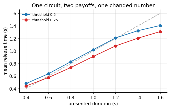
neural shift (theta 0.5 minus 0.25): [0.039 0.06 0.093 0.108 0.127 0.119 0.097]
Stage 6 · Prediction and failure
prediction how to test rejected if The shift follows the width of the belief: it grows with duration and levels off at the prior edge. asymmetric vs symmetric blocks, several durations the shift is flat (a fixed “press earlier” rule) The quantile follows the cost ratio, \(q = c_\text{early} / (c_\text{early} + c_\text{late})\). blocks with ratios 1:3, 1:1, 3:1 shifts do not order with \(q\), or saturate early Noisier timers shift more. individual differences in \(\sigma_w\) from the symmetric block shift size is unrelated to fitted \(\sigma_w\) Mean and median are not separable in this design. model recovery before running the study (a design property, not a hypothesis) half = rng.permutation(s_asy.size)
train, test = half[: s_asy.size // 2], half[s_asy.size // 2:]
def nll_actions(a_of_m, s, r, sw, s_mot):
W = norm.pdf(np.log(m_grid)[None, :], np.log(s)[:, None], sw)
W /= W.sum(axis=1, keepdims=True) # (N, M)
return -np.log((W * norm.pdf(r[:, None], a_of_m[None, :], s_mot)).sum(axis=1) + 1e-300).sum()
# Rival: constant offset, delta fitted on the training half
deltas = np.linspace(0, 0.3, 61)
train_nll = [nll_actions(a_mean - d, s_asy[train], r_asy[train], sw_hat, mot_hat) for d in deltas]
delta_hat = deltas[int(np.argmin(train_nll))]
test_quant = nll_actions(a_q, s_asy[test], r_asy[test], sw_hat, mot_hat)
test_offset = nll_actions(a_mean - delta_hat, s_asy[test], r_asy[test], sw_hat, mot_hat)
print(f"fitted offset delta = {delta_hat:.3f} s")
print(f"held out -log L: quantile model {test_quant:.1f}, constant offset {test_offset:.1f}")
print(f"difference {test_offset - test_quant:.1f} in favor of the "
f"{'quantile' if test_quant < test_offset else 'offset'} model")
fig, ax = plt.subplots(figsize=(6, 3.4))
ax.errorbar(durs, shift, yerr=se_shift, fmt="o", color="k", capsize=3, label="data")
ax.plot(durs, pred_shift, color="C3", lw=2, label="quantile (0 free parameters)")
ax.axhline(delta_hat, color="C0", lw=2, ls="--", label="constant offset (1 free parameter)")
ax.set(xlabel="presented duration (s)", ylabel="symmetric minus asymmetric (s)", title="Two accounts of the shift")
ax.legend(frameon=False, fontsize=8)
plt.show()
fitted offset delta = 0.070 s
held out -log L: quantile model -159.2, constant offset -151.0
difference 8.3 in favor of the quantile model
What to carry forward
joint = lik * prior[:, None], post = joint / joint.sum(0). Shapes first.References